机器学习算法系列之线性回归

最新推荐文章于 2022-06-01 17:39:51 发布

L轻描淡写L

最新推荐文章于 2022-06-01 17:39:51 发布

阅读量504

点赞数

分类专栏：机器学习

本文链接：https://blog.csdn.net/qq_41999763/article/details/105922221

版权

机器学习专栏收录该内容

6 篇文章 0 订阅

订阅专栏

本系列机器学习的文章打算从机器学习算法的一些理论知识、python实现该算法和调一些该算法的相应包来实现。

线性回归

一、理论知识

1、什么是线性回归

2、线性回归一般表达式及最小二乘法计算损失

3、正则化

二、python代码实现线性回归模型

三、使用sklearn实现线性回归模型

线性回归

一、理论知识

1、什么是线性回归

线性：两个变量之间的关系是一次函数的关系的----图像是直线，叫做线性

非线性：两个变量之间不是一次函数关系的----图像不是直线，叫做非线性

回归：人们在测量事物的时候因为客观条件有限，求得得都是测量值，而不是事物得真实值，为了能够得到真实值，无限次的进行测量，最后从这些测量数据中计算回归到真实值，这就是回归的由来。（从数据中计算得到规律）

回归问题的学习等价于函数拟合：选择一条函数曲线很好地拟合已知数据且很好地预测未知数据。

其线性回归解决的一般就是通过已知数据得到未知的结果，例如在收集到一些房子的数据和对应的价格后，利用线性回归去预测未知的房价。

2、线性回归一般表达式及最小二乘法计算损失

一般表达式：Y=WX+b 其中：W叫做X的系数，b叫做偏置项。此时拟合出来的图像时一条直线，如图

当数据扩展到多维时： ${h_\theta }(x) = {\theta _0} + {\theta _1}{x_1} + {\theta _2}{x_2} + ...$ 此时拟合出地不再是一条直线，而是一个超平面。

最小二乘法（LS）：利用梯度下降法找到最小值点，也就是最小误差，最后把 w 和 b 给求出来

3、正则化

在机器学习中加入正则化项能有效的解决过拟合和欠拟合的问题，这里介绍两种正则化：L1正则化和L2正则化

L1正则化
L1正则化（Lasso回归）：直接在原来的损失函数基础上加上权重参数的绝对值。
方程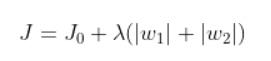：其中 $\lambda$ 是正则化参数，可调。
使用场景：L1正则化可以使得一些特征得系数变小，甚至还使得一些较小得系数直接变为0，从而增强模型得泛化能力。
对于一些高的特征数据，尤其是线性关系是稀疏的，就采用L1正则化，或者是要在一堆特征里面找出主要的特征。
L2正则化
L2正则化（岭回归）：直接在原来的模型损失函数上加上权重参数的平方和。
方程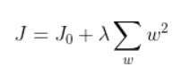：其中 $\lambda$ 是正则化参数，可调。

使用场景：只要数据线性相关，用线性回归拟合的不是很好，需要正则化。可以考虑用L2（岭回归），如果输入特征值的维度很高，而且是稀疏线性相关的话，岭回归就不太合适，考虑使用L1正则化（Lasso回归）。

注意：在用线性回归模型拟合数据之前，首先要求数据应符合或则近似符合正态分布，否则得到的拟合函数将会不准确。

二、python代码实现线性回归模型

数据介绍
这里简单的使用房价数据中的两个参数房子的每平米单价和房间的数量

2104,3,399900
1600,3,329900
2400,3,369000
1416,2,232000
3000,4,539900
1985,4,299900
1534,3,314900
1427,3,198999
1380,3,212000
1494,3,242500
1940,4,239999
2000,3,347000
1890,3,329999
4478,5,699900
1268,3,259900
2300,4,449900
1320,2,299900
1236,3,199900
2609,4,499998
3031,4,599000
1767,3,252900
1888,2,255000
1604,3,242900
1962,4,259900
3890,3,573900
1100,3,249900
1458,3,464500
2526,3,469000
2200,3,475000
2637,3,299900
1839,2,349900
1000,1,169900
2040,4,314900
3137,3,579900
1811,4,285900
1437,3,249900
1239,3,229900
2132,4,345000
4215,4,549000
2162,4,287000
1664,2,368500
2238,3,329900
2567,4,314000
1200,3,299000
852,2,179900
1852,4,299900
1203,3,239500

python代码：

# -*- coding: utf-8 -*-
from __future__ import print_function
import numpy as np
from matplotlib import pyplot as plt
from matplotlib.font_manager import FontProperties
from mpl_toolkits.mplot3d import Axes3D
font = FontProperties(fname=r"c:\windows\fonts\simsun.ttc", size=14)  # 解决windows环境下画图汉字乱码问题


def linearRegression(alpha=0.01, num_iters=400):
    print(u"加载数据...\n")

    data = loadtxtAndcsv_data("data.txt", ",", np.float64)  # 读取数据
    X = data[:, 0:-1]  # X对应0到倒数第2列
    y = data[:, -1]  # y对应最后一列
    m = len(y)  # 总的数据条数
    col = data.shape[1]  # data的列数
    plot_X_y(X,y)
    X, mu, sigma = featureNormaliza(X)  # 归一化
    plot_X1_X2(X)  # 画图看一下归一化效果

    X = np.hstack((np.ones((m, 1)), X))  # 在X前加一列1

    print(u"\n执行梯度下降算法....\n")

    theta = np.zeros((col, 1))
    y = y.reshape(-1, 1)  # 将行向量转化为列
    theta, J_history = gradientDescent(X, y, theta, alpha, num_iters)

    plotJ(J_history, num_iters)

    return mu, sigma, theta  # 返回均值mu,标准差sigma,和学习的结果theta


# 加载txt和csv文件
def loadtxtAndcsv_data(fileName, split, dataType):
    return np.loadtxt(fileName, delimiter=split, dtype=dataType)


# 加载npy文件
def loadnpy_data(fileName):
    return np.load(fileName)


# 归一化feature
def featureNormaliza(X):
    X_norm = np.array(X)  # 将X转化为numpy数组对象，才可以进行矩阵的运算
    # 定义所需变量
    mu = np.zeros((1, X.shape[1]))
    sigma = np.zeros((1, X.shape[1]))

    mu = np.mean(X_norm, 0)  # 求每一列的平均值（0指定为列，1代表行）
    sigma = np.std(X_norm, 0)  # 求每一列的标准差
    for i in range(X.shape[1]):  # 遍历列
        X_norm[:, i] = (X_norm[:, i] - mu[i]) / sigma[i]  # 归一化

    return X_norm, mu, sigma

# 画数据分布图
def plot_X_y(X,y):
    ax = plt.subplot(111,projection ='3d')
    ax.scatter(X[:, 0], X[:, 1],y)
    plt.show()


# 画二维图
def plot_X1_X2(X):
    plt.scatter(X[:, 0], X[:, 1])
    plt.show()


# 梯度下降算法
def gradientDescent(X, y, theta, alpha, num_iters):
    m = len(y)
    n = len(theta)

    temp = np.matrix(np.zeros((n, num_iters)))  # 暂存每次迭代计算的theta，转化为矩阵形式

    J_history = np.zeros((num_iters, 1))  # 记录每次迭代计算的代价值

    for i in range(num_iters):  # 遍历迭代次数
        h = np.dot(X, theta)  # 计算内积，matrix可以直接乘
        temp[:, i] = theta - ((alpha / m) * (np.dot(np.transpose(X), h - y)))  # 梯度的计算
        theta = temp[:, i]
        J_history[i] = computerCost(X, y, theta)  # 调用计算代价函数
        print('.', end=' ')
    return theta, J_history


# 计算代价函数
def computerCost(X, y, theta):
    m = len(y)
    J = 0

    J = (np.transpose(X * theta - y)) * (X * theta - y) / (2 * m)  # 计算代价J
    return J


# 画每次迭代代价的变化图
def plotJ(J_history, num_iters):
    x = np.arange(1, num_iters + 1)
    plt.plot(x, J_history)
    plt.xlabel(u"迭代次数", fontproperties=font)  # 注意指定字体，要不然出现乱码问题
    plt.ylabel(u"代价值", fontproperties=font)
    plt.title(u"代价随迭代次数的变化", fontproperties=font)
    plt.show()

#绘制回归曲面的图像
# def regressionImg(X,theta):
#     y=np.matrix(X,theta);

# 测试linearRegression函数
def testLinearRegression():
    mu, sigma, theta = linearRegression(0.01, 400)
    print(u"\n计算的theta值为：\n",theta)
    print(u"\n预测结果为：%f"%predict(mu, sigma, theta))


# 测试学习效果（预测）
def predict(mu, sigma, theta):
    result = 0
    # 注意归一化
    predict = np.array([1650, 3])
    norm_predict = (predict - mu) / sigma
    final_predict = np.hstack((np.ones((1)), norm_predict))

    result = np.dot(final_predict, theta)  # 预测结果
    return result


if __name__ == "__main__":
    testLinearRegression()

代码执行效果图和损失函数曲线图：

三、使用sklearn实现线性回归模型

数据说明：数据主要包括2014年5月至2015年5月美国King County的房屋销售价格以及房屋的基本信息。数据分为训练数据和测试数据，分别保存在kc_train.csv和kc_test.csv两个文件中。其中训练数据主要包括10000条记录，14个字段，主要字段说明如下：第一列“销售日期”：2014年5月到2015年5月房屋出售时的日期第二列“销售价格”：房屋交易价格，单位为美元，是目标预测值第三列“卧室数”：房屋中的卧室数目第四列“浴室数”：房屋中的浴室数目第五列“房屋面积”：房屋里的生活面积第六列“停车面积”：停车坪的面积第七列“楼层数”：房屋的楼层数第八列“房屋评分”：King County房屋评分系统对房屋的总体评分第九列“建筑面积”：除了地下室之外的房屋建筑面积第十列“地下室面积”：地下室的面积第十一列“建筑年份”：房屋建成的年份第十二列“修复年份”：房屋上次修复的年份第十三列"纬度"：房屋所在纬度第十四列“经度”：房屋所在经度
测试数据主要包括3000条记录，13个字段，跟训练数据的不同是测试数据并不包括房屋销售价格，学员需要通过由训练数据所建立的模型以及所给的测试数据，得出测试数据相应的房屋销售价格预测值
数据集下载：https://pan.baidu.com/share/init?surl=kVdwI3d 密码：mfqy

代码：

# -*- coding:UTF-8 -*-
# 兼容 pythone2,3

from __future__ import print_function

# 导入相关python库
import os
import numpy as np
import pandas as pd

# 设定随机数种子
np.random.seed(36)

# 使用matplotlib库画图

import matplotlib

import seaborn
import matplotlib.pyplot as plot
from sklearn import datasets

# 读取数据
housing = pd.read_csv('kc_train.csv')

target = pd.read_csv('kc_train2.csv')  # 销售价格

t = pd.read_csv('kc_test.csv')  # 测试数据

# 数据预处理

housing.info()  # 查看是否有缺失值

# 特征缩放
from sklearn.preprocessing import MinMaxScaler

minmax_scaler = MinMaxScaler()
minmax_scaler.fit(housing)  # 进行内部拟合，内部参数会发生变化
scaler_housing = minmax_scaler.transform(housing)
scaler_housing = pd.DataFrame(scaler_housing, columns=housing.columns)
mm = MinMaxScaler()
mm.fit(t)
scaler_t = mm.transform(t)
scaler_t = pd.DataFrame(scaler_t, columns=t.columns)

# 选择基于梯度下降的线性回归模型

from sklearn.linear_model import LinearRegression

LR_reg = LinearRegression()

# 进行拟合
LR_reg.fit(scaler_housing, target)

# 使用均方误差用于评价模型好坏

from sklearn.metrics import mean_squared_error

preds = LR_reg.predict(scaler_housing)  # 输入数据进行预测得到结果
mse = mean_squared_error(preds, target)  # 使用均方误差来评价模型好坏，可以输出mse进行查看评价值

# 绘图进行比较
plot.figure(figsize=(10, 7))  # 画布大小
num = 100
x = np.arange(1, num + 1)  # 取100个点进行比较
plot.plot(x, target[:num], label='target')  # 目标取值
plot.plot(x, preds[:num], label='preds')  # 预测取值
plot.legend(loc='upper right')  # 线条显示位置
plot.show()

# 输出测试数据

result = LR_reg.predict(scaler_t)

df_result = pd.DataFrame(result)

df_result.to_csv("result.csv")

输出拟合图像

参考：《统计学习方法》 ——李航

https://github.com/NLP-LOVE/ML-NLP/tree/master/Machine%20Learning/Liner%20Regression

L轻描淡写L

关注

0
点赞
踩
2

收藏

觉得还不错? 一键收藏
0
评论
机器学习算法系列之线性回归

本系列机器学习的文章打算从机器学习算法的一些理论知识、python实现该算法和调一些该算法的相应包来实现。线性回归一、理论知识1、什么是线性回归线性：两个变量之间的关系是一次函数的关系的----图像是直线，叫做线性非线性：两个变量之间不是一次函数关系的----图像不是直线，叫做非线性回归：人们在测量事物的时候因为客观条件有限，求得得都是测量值，而不是事物得真实值，为了能够得...
复制链接

扫一扫