机器学习——Adaline自适应线性神经元（适合初学者，注释明确细致）

机器学习——Adaline自适应线性神经元（适合初学者，注释明确细致）

参考书

Python机器学习【美】 塞巴斯蒂安.拉托卡

运行环境

windows10—pycharm——python3.8.10

运行结果

代码及运行步骤

先在工程中保存以下文件，文件名设置为jiandu.py

import numpy as np


"""线性神经元  python机器学习 第21页"""


class AdalineGD(object):
    """ADAptive LInear NEuron classifier

    parameter
    _________
    eta :float
        Learning rate (between 0.0 and 1.0)
    n_iter : int
        Passes over the training dataset.
        迭代次数

    Attributes
    ___________
    w_ :ld-array
        Weights after  fitting.
    errors_ :list
        Number of misclassifications in every epoch.

    """
    # 初始化函数 eta：学习速率 n_iter：迭代次数
    def __init__(self, eta=0.01, n_iter=50):
        self.eta = eta
        self.n_iter = n_iter

    # fit 拟合 输入：样本+样本对应的特征
    def fit(self, x, y):
        """Fit training data.

        :param x:{array-like}, shape = [n_samples, n_features]
        Training vectors, where n_sample is the number of samples and
        n_feature is the number of features

        :param y:array-like, shape = [n_samples]
        Target values.

        :return:
        self : object

        """
        self.w_ = np.zeros(1 + x.shape[1])
        self.cost_ = []  # 代价函数

        for i in range(self.n_iter):
            output = self.net_input(x)  # 该算法下：激励函数输出 = 净输入
            errors = (y - output)
            self.w_[1:] += self.eta * x.T.dot(errors)  # .T：矩阵转置
            self.w_[0] += self.eta * errors.sum()  # ? w[0] 为基础值
            cost = (errors**2).sum() / 2.0  # 误差平方和 SSE
            self.cost_.append(cost)  # 储存代价函数输出值，检验本轮训练后是否收敛
        return self

    def net_input(self, x):  # 净输入函数
        """Calculate net input"""
        return np.dot(x, self.w_[1:]) + self.w_[0]

    def activation(self, x):
        """Compute linear activation"""
        return self.net_input(x)

    def predict(self, x):   # 量化器
        """return class label after unit step"""
        return np.where(self.activation(x) >= 0.0, 1, -1)

再运行主程序

import pandas as pd
import matplotlib.pyplot as plt
import numpy as np
from jiandu import AdalineGD
from matplotlib.colors import ListedColormap
from mlxtend.plotting import plot_decision_regions


"""数据录入"""
df = pd.read_csv('https://archive.ics.uci.edu/ml/machine-learning-databases/iris/iris.data',header=None)
# 原数据无表头，header=None保障第一行数据不会自动成为表头
y = df.iloc[0:100, 4].values
y = np.where(y == 'Iris-setosa',-1,1)  # 打标签
x = df.iloc[0:100, [0, 2]].values


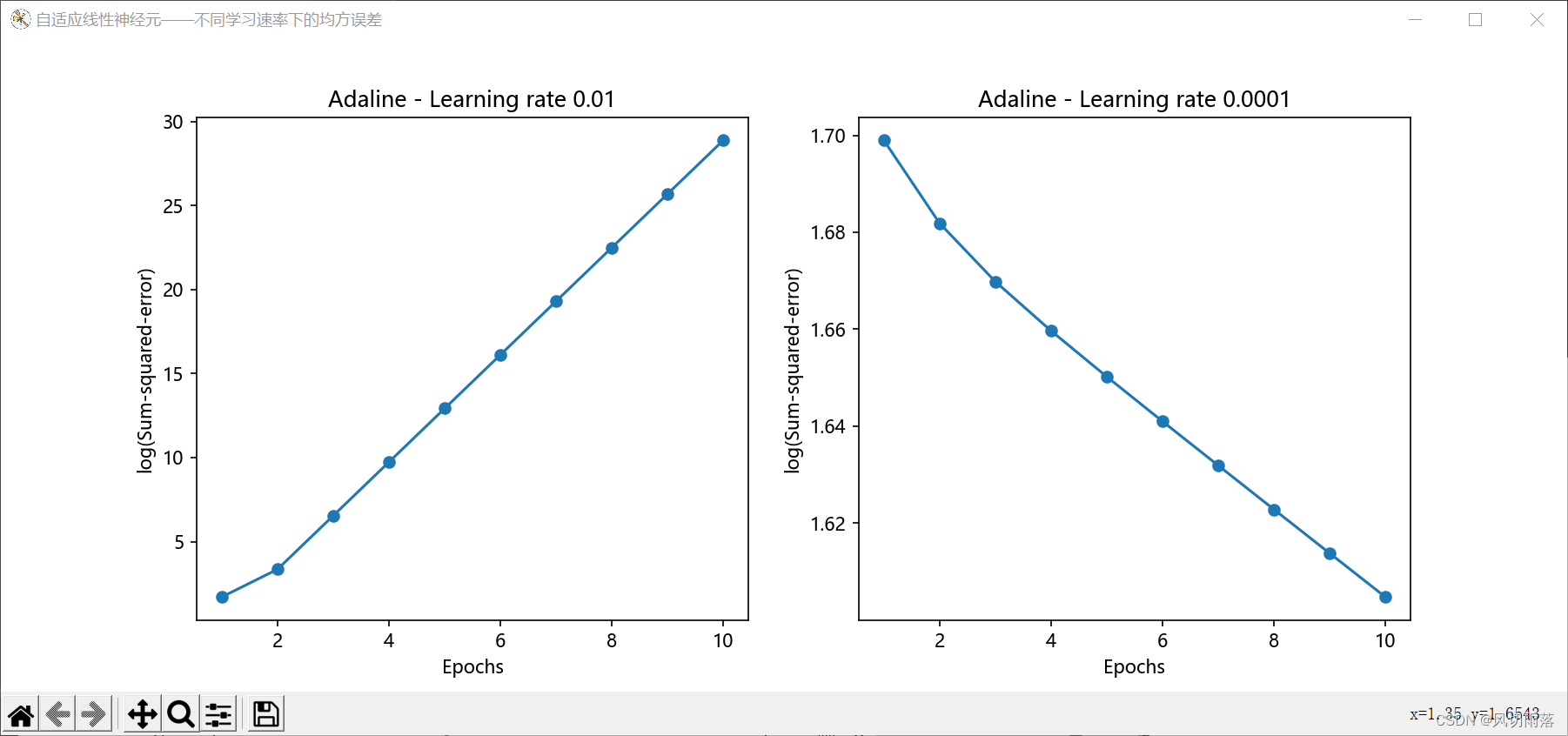
"""自适应线性神经元，不同学习速率下的均方误差"""
ax = plt.figure(num='自适应线性神经元——不同学习速率下的均方误差', figsize=(12, 5)).subplots(nrows=1, ncols=2)
plt.subplots_adjust()
plt.rcParams['font.sans-serif'] =['Microsoft YaHei']
plt.rcParams['axes.unicode_minus'] = False

ada1 = AdalineGD(n_iter=10, eta=0.01).fit(x, y)
ax[0].plot(range(1, len(ada1.cost_) + 1),
           np.log10(ada1.cost_), marker='o')
ax[0].set_xlabel('Epochs')
ax[0].set_ylabel('log(Sum-squared-error)')
ax[0].set_title('Adaline - Learning rate 0.01')

ada2 = AdalineGD(n_iter=10, eta=0.0001).fit(x, y)
ax[1].plot(range(1, len(ada2.cost_) + 1),
           np.log10(ada2.cost_), marker='o')
ax[1].set_xlabel('Epochs')
ax[1].set_ylabel('log(Sum-squared-error)')
ax[1].set_title('Adaline - Learning rate 0.0001')


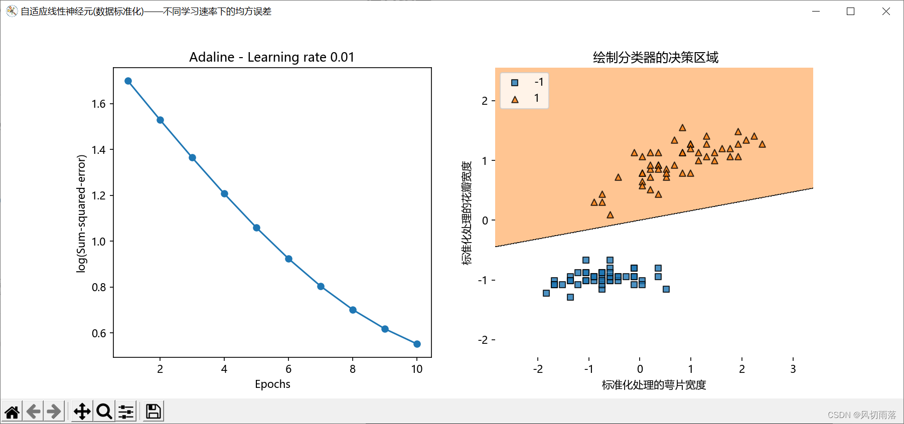
"""数据特征标准化处理"""
x_biao = np.copy(x)
x_biao[:, 0] = (x[:, 0]-x[:, 0].mean()) / x[:, 0].std()
x_biao[:, 1] = (x[:, 1]-x[:, 1].mean()) / x[:, 1].std()

# 绘图
ax = plt.figure(num='自适应线性神经元(数据标准化)——不同学习速率下的均方误差', figsize=(12, 5)).subplots(nrows=1, ncols=2)
plt.rcParams['font.sans-serif'] =['Microsoft YaHei']
plt.rcParams['axes.unicode_minus'] = False

ada1 = AdalineGD(n_iter=10, eta=0.01).fit(x_biao, y)
ax[0].plot(range(1, len(ada1.cost_) + 1),
           np.log10(ada1.cost_), marker='o')
ax[0].set_xlabel('Epochs')
ax[0].set_ylabel('log(Sum-squared-error)')
ax[0].set_title('Adaline - Learning rate 0.01')

plot_decision_regions(x_biao, y, clf=ada1)  # 绘制分类器的决策区域
ax[1].set_xlabel('标准化处理的萼片宽度')
ax[1].set_ylabel('标准化处理的花瓣宽度')
ax[1].set_title(' 绘制分类器的决策区域')
ax[1].legend(loc='upper left')  # 标签位置设置

"""绘图"""
plt.show()


"""
结果注释：
若不进行数据标准化处理
图（1，2，1）：代价函数随学习次数越来越大，是因为跳过了全局最优解
"""