


Gradient Boosting
以梯度为优化目标,以提升将整个架构串在一起,用决策树当做模型细节中的每一个小部分
分类回归树(CART)
数据集: { ( ( x ( 1 ) , y ( 1 ) ) , ( x ( 2 ) , y ( 2 ) ) , . . . , ( x ( m ) , y ( m ) ) ) } \begin{Bmatrix} ((x^{(1)},y^{(1)}),(x^{(2)},y^{(2)}),...,(x^{(m)},y^{(m)})) \end{Bmatrix} {((x(1),y(1)),(x(2),y(2)),...,(x(m),y(m)))}
衡量标准:
s 2 ⋅ m = ( y ( 1 l e f t ) − y ˉ l e f t ) 2 + . . . + ( y ( n l e f t ) − y ˉ l e f t ) 2 + ( y ( 1 r i g h t ) − y ˉ r i g h t ) 2 + . . . + ( y ( m − n l e f t ) − y ˉ r i g h t ) 2 s^2 \cdot m= (y^{(1_{left})}-\bar{y}_{left})^2+...+(y^{(n_{left})}-\bar{y}_{left})^2+(y^{(1_{right})}-\bar{y}_{right})^2+...+(y^{(m-n_{left})}-\bar{y}_{right})^2 s2⋅m=(y(1left)−yˉleft)2+...+(y(nleft)−yˉleft)2+(y(1right)−yˉright)2+...+(y(m−nleft)−yˉright)2
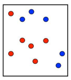
Adaboost算法概述
原数据集:
第一次划分:
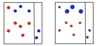
在第一次划分完成后,对于分类正确的数据降低权重,分类错误的值增加权重
第二次划分:
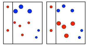
在第二次划分完成后,同样是对于分类正确的数据降低权重,分类错误的值增加权重
第三次划分:
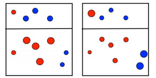
在第三次划分完成后,同样是做权重调整工作
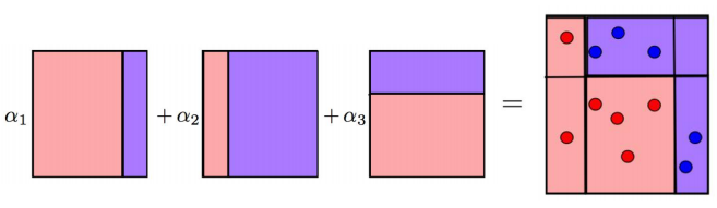
最终,对三次分类进行整合,不同的分类精度对应不同的
α
\alpha
α 权重,将其加和得到最后结果
GB算法
优化的目标:
a
r
g
m
i
n
f
(
x
)
E
x
,
y
[
L
(
y
,
f
(
x
)
)
]
\underset{f(x)}{arg min}E_{x,y}[L(y,f(x))]
f(x)argminEx,y[L(y,f(x))]
L ( y , f ( x ) ) L(y,f(x)) L(y,f(x))是一个损失函数, f ( x ) f(x) f(x) 是一个模型,我们需要找到一个模型 f ( x ) f(x) f(x) 使得损失函数最小
其实目标还是去找最合适的参数:
θ
^
=
a
r
g
m
i
n
θ
E
x
,
y
[
L
(
y
,
f
(
x
,
θ
)
)
]
\hat{\theta} =\underset{\theta }{arg min}E_{x,y}[L(y,f(x,\theta ))]
θ^=θargminEx,y[L(y,f(x,θ))]
结果依旧是需要迭代得出:
θ
^
=
∑
i
=
1
M
θ
^
i
\hat{\theta} = \sum_{i=1}^{M}\hat{\theta}_i
θ^=i=1∑Mθ^i
梯度的思想
找到最合适的参数:
(
ρ
t
,
θ
t
)
=
a
r
g
m
i
n
ρ
,
θ
E
x
,
y
[
L
(
y
,
f
^
(
x
)
+
ρ
⋅
h
(
x
,
θ
)
)
]
(\rho _t,\theta _t)=\underset{\rho ,\theta }{argmin}E_{x,y}[L(y,\hat{f}(x )+\rho \cdot h(x,\theta))]
(ρt,θt)=ρ,θargminEx,y[L(y,f^(x)+ρ⋅h(x,θ))]
残差的计算(负梯度):
r
i
t
=
−
[
∂
L
(
y
,
f
(
x
i
)
)
∂
f
(
x
i
)
]
f
(
x
i
)
=
f
^
(
x
)
r_{it}=-[\frac{\partial L(y,f(x_i))}{\partial f(x_i)}]_{f(x_i)=\hat{f}(x )}
rit=−[∂f(xi)∂L(y,f(xi))]f(xi)=f^(x)
参数迭代:
θ
t
=
a
r
g
m
i
n
θ
∑
i
=
1
n
(
r
i
t
−
h
(
x
i
,
θ
)
)
2
\theta _t=\underset{\theta }{argmin}\sum_{i=1}^{n}(r_{it}-h(x_i,\theta))^2
θt=θargmini=1∑n(rit−h(xi,θ))2
步长的选择:
ρ
t
=
a
r
g
m
i
n
ρ
∑
i
=
1
n
L
(
y
i
,
f
^
(
x
i
)
+
ρ
⋅
h
(
x
i
,
θ
t
)
)
\rho _t=\underset{\rho }{argmin}\sum_{i=1}^{n}L(y_i,\hat{f}(x_i)+\rho \cdot h(x_i,\theta_t))
ρt=ρargmini=1∑nL(yi,f^(xi)+ρ⋅h(xi,θt))
GBDT的工作流程 { ( x i , y i ) } i = 1 , . . . , n \begin{Bmatrix}(x_i,y_i) \end{Bmatrix}_{i=1,...,n} {(xi,yi)}i=1,...,n
关于GBDT的工作流程,假设100个数据在一次训练迭代了三次模型,分别为 f 1 ( x ) , f 2 ( x ) , f 3 ( x ) f_1{(x)},f_2{(x)},f_3{(x)} f1(x),f2(x),f3(x),第一个模型 f 1 ( x ) f_1{(x)} f1(x) 拟合了 80 % 80\% 80% 的精度,那么在第二次拟合时,第二个模型 f 2 ( x ) f_2{(x)} f2(x) 以剩下的 20 % 20\% 20% 的精度为基础继续进行训练拟合了 18 % 18\% 18% 的精度,第三个模型 f 3 ( x ) f_3{(x)} f3(x) 继续以剩下的 2 % 2\% 2% 的精度进行训练,拟合掉了 1 % 1\% 1% ,那么到最后这三个模型就是以这样的拟合占比进行相加,得到最终 99 % 99\% 99% 正确率的结果
- 初始化第一个方程:
f ^ ( x ) = f ^ 0 , f ^ 0 = γ , γ ∈ R , f ^ 0 = a r g m i n γ L ( y i , γ ) \hat{f}(x)=\hat{f}_0,\hat{f}_0=\gamma ,\gamma \in R,\hat{f}_0=\underset{\gamma}{arg min}L(y_i,\gamma) f^(x)=f^0,f^0=γ,γ∈R,f^0=γargminL(yi,γ) - 每次迭代都要计算残差:
r i t = − [ ∂ L ( y , f ( x i ) ) ∂ f ( x i ) ] f ( x i ) = f ^ ( x ) , i = 1 , . . . , n r_{it}=-[\frac{\partial L(y,f(x_i))}{\partial f(x_i)}]_{f(x_i)=\hat{f}(x )},i =1,...,n rit=−[∂f(xi)∂L(y,f(xi))]f(xi)=f^(x),i=1,...,n - 以残差为目标构建回归方程:
{ ( x i , r i t ) } i = 1 , . . . , n \begin{Bmatrix}(x_i,r_{it}) \end{Bmatrix}_{i=1,...,n} {(xi,rit)}i=1,...,n - 找到当前最合适的组合(遍历):
ρ t = a r g m i n ρ ∑ i = 1 n L ( y i , f ^ ( x i ) + ρ ⋅ h ( x i , θ t ) ) \rho _t=\underset{\rho }{argmin}\sum_{i=1}^{n}L(y_i,\hat{f}(x_i)+\rho \cdot h(x_i,\theta_t)) ρt=ρargmini=1∑nL(yi,f^(xi)+ρ⋅h(xi,θt)) - 经过M次迭代后的结果:
∑ i = 0 M f ^ i ( x ) \sum_{i=0}^{M}\hat{f}_i(x) i=0∑Mf^i(x)
GBDT的回归任务

以这张图为例,在第一次回归后得到的残差,放入第二个回归树模型中再次进行回归任务
A
的
预
测
值
=
树
1
左
节
点
(
值
15
)
+
树
2
左
节
点
(
值
−
1
)
=
14
B
的
预
测
值
=
树
1
左
节
点
(
值
15
)
+
树
2
右
节
点
(
值
−
1
)
=
16
C
的
预
测
值
=
树
1
右
节
点
(
值
25
)
+
树
2
左
节
点
(
值
−
1
)
=
24
D
的
预
测
值
=
树
1
右
节
点
(
值
25
)
+
树
2
右
节
点
(
值
−
1
)
=
26
A的预测值=树1左节点(值15)+树2左节点(值-1)=14 \\ B的预测值=树1左节点(值15)+树2右节点(值-1)=16 \\ C的预测值=树1右节点(值25)+树2左节点(值-1)=24 \\ D的预测值=树1右节点(值25)+树2右节点(值-1)=26
A的预测值=树1左节点(值15)+树2左节点(值−1)=14B的预测值=树1左节点(值15)+树2右节点(值−1)=16C的预测值=树1右节点(值25)+树2左节点(值−1)=24D的预测值=树1右节点(值25)+树2右节点(值−1)=26
GBDT的分类任务
分类与回归任务均使用CART,原理和多分类的逻辑回归类似,使用GBDT得到类别的概率值,对应进行分类。比如一个三分类问题,我们可以训练3颗树(分别表示是不是第一类,是不是第二类,是不是第三类)
分类任务实例
假设当前样本属于第二类(第一轮,输入的为真实值): { f 11 ( x ) = 0 − f 1 ( x ) f 22 ( x ) = 1 − f 1 ( x ) f 33 ( x ) = 0 − f 1 ( x ) \left\{\begin{matrix} f_{11}(x)=0-f_1(x)\\ f_{22}(x)=1-f_1(x)\\ f_{33}(x)=0-f_1(x) \end{matrix}\right. ⎩⎨⎧f11(x)=0−f1(x)f22(x)=1−f1(x)f33(x)=0−f1(x)
第二轮输入: ( x , f 11 ( x ) ) , ( x , f 22 ( x ) ) , ( x , f 33 ( x ) ) (x,f_{11}(x)),(x,f_{22}(x)),(x,f_{33}(x)) (x,f11(x)),(x,f22(x)),(x,f33(x))
最后进行归一化
p
2
=
e
x
p
(
f
1
(
x
)
)
∑
k
=
1
3
e
x
p
(
f
k
(
x
)
)
p_2=\frac{exp(f_1(x))}{\sum_{k=1}^{3}exp(f_k(x))}
p2=∑k=13exp(fk(x))exp(f1(x))
可视化解释
GBDT、Xgboost、LightGBM对比
Mnist数据集识别
使用Sklearn的GBDT
GradientBoostingClassifier
GradientBoostingRegressor
import gzip
import pickle as pkl
from sklearn.model_selection import train_test_split
# 读文件划分数据集
def load_data(path):
    f = gzip.open(path, 'rb')
    try:
        #Python3
        train_set, valid_set, test_set = pkl.load(f, encoding='latin1')
    except:
        #Python2
        train_set, valid_set, test_set = pkl.load(f)
    f.close()
    return(train_set,valid_set,test_set)

path = 'mnist.pkl.gz'
train_set,valid_set,test_set = load_data(path)

Xtrain,_,ytrain,_ = train_test_split(train_set[0], train_set[1], test_size=0.9)
Xtest,_,ytest,_ = train_test_split(test_set[0], test_set[1], test_size=0.9)
print(Xtrain.shape, ytrain.shape, Xtest.shape, ytest.shape)
参数说明:
- learning_rate: The learning parameter controls the magnitude of this change in the estimates. (default=0.1)
- n_extimators: The number of sequential trees to be modeled. (default=100)
- max_depth: The maximum depth of a tree. (default=3)
- min_samples_split: Tthe minimum number of samples (or observations) which are required in a node to be considered for splitting. (default=2)
- min_samples_leaf: The minimum samples (or observations) required in a terminal node or leaf. (default=1)
- min_weight_fraction_leaf: Similar to min_samples_leaf but defined as a fraction of the total number of observations instead of an integer. (default=0.)
- subsample: The fraction of observations to be selected for each tree. Selection is done by random sampling. (default=1.0)
- max_features: The number of features to consider while searching for a best split. These will be randomly selected. (default=None)
- max_leaf_nodes: The maximum number of terminal nodes or leaves in a tree. (default=None)
- min_impurity_decrease: A node will be split if this split induces a decrease of the impurity greater than or equal to this value. (default=0.)
实例测试:
from sklearn.ensemble import GradientBoostingClassifier
import numpy as np
import time
# 实例化
clf = GradientBoostingClassifier(n_estimators=10,
                                 learning_rate=0.1,
                                 max_depth=3)
# 开始训练,记录时间
start_time = time.time()
clf.fit(Xtrain, ytrain)
end_time = time.time()
print('The training time = {}'.format(end_time - start_time))
# 预测与评价
pred = clf.predict(Xtest)
accuracy = np.sum(pred == ytest) / pred.shape[0]
print('Test accuracy = {}'.format(accuracy))
The training time = 27.277734518051147
Test accuracy = 0.815
集成算法可以得出特征重要性,这里画图看一下
import matplotlib.pyplot as plt
# 得到特征重要性结果 画图
plt.hist(clf.feature_importances_)

一般情况下,我们还要根据特征重要性进行筛选,将有用的特征保留
from collections import OrderedDict
# 选出重要性>0.01的特征
d = {}
for i in range(len(clf.feature_importances_)):
    if clf.feature_importances_[i] > 0.01:
        d[i] = clf.feature_importances_[i]
# 重要性排序
sorted_feature_importances = OrderedDict(sorted(d.items(), key=lambda x:x[1], reverse=True))
D = sorted_feature_importances
# 画图
rects = plt.bar(range(len(D)), D.values(), align='center')
plt.xticks(range(len(D)), D.keys(),rotation=90)
plt.show()

XGBoost
XGBoost 加入了更多的剪枝策略和正则项,控制过拟合风险。传统的GBDT用的是CART,Xgboost能支持的分类器更多,也可以是线性的。GBDT只用了一阶导,但是xgboost对损失函数做了二阶的泰勒展开,并且还可以自定义损失函数。
import xgboost as xgb
import numpy as np
import time

# 数据读入Xgboost DMatrix格式
dtrain = xgb.DMatrix(Xtrain, label=ytrain)
dtest = xgb.DMatrix(Xtest, label=ytest)

# 通过映射指定参数
params = {
    'booster':'gbtree',     #  tree-based models
    'objective': 'multi:softmax',
    'num_class':10,
    'eta': 0.1,             # Same to learning rate in GBDT
    'gamma':0,              # Similar to min_impurity_decrease in GBDT
    'alpha': 0,             # L1 regularization term on weight (analogous to Lasso regression)
    'lambda': 2,            # L2 regularization term on weights (analogous to Ridge regression)
    'max_depth': 3,         # Same as the max_depth of GBDT
    'subsample': 1,         # Same as the subsample of GBDT
    'colsample_bytree': 1,  # Similar to max_features in GBM
    'min_child_weight': 1,  # minimum sum of instance weight (Hessian) needed in a child
    'nthread':1,            # default to maximum number of threads available if not set
}
num_round = 10

# 开始训练,记录时间
start_time = time.time()
bst = xgb.train(params, dtrain, num_round)
end_time = time.time()
print('The training time = {}'.format(end_time - start_time))

# 预测与评价
ypred = bst.predict(dtest)
accuracy = np.sum(ypred == ytest) / ypred.shape[0]
print('Test accuracy = {}'.format(accuracy))
The training time = 15.998175859451294
Test accuracy = 0.827
LightGBM
优点:
-
更快的训练效率
-
低内存使用
-
更好的准确率
-
支持并行学习
-
可处理大规模数据
它摒弃了现在大部分GBDT使用的按层生长(level-wise)的决策树生长策略,使用带有深度限制的按叶子生长(leaf-wise)的策略。level-wise过一次数据可以同时分裂同一层的叶子,容易进行多线程优化,也好控制模型复杂度,不容易过拟合。但实际上level-wise是一种低效的算法,因为它不加区分的对待同一层的叶子,带来了很多没必要的开销,因为实际上很多叶子的分裂增益较低,没必要进行搜索和分裂。

Leaf-wise则是一种更为高效的策略,每次从当前所有叶子中,找到分裂增益最大的一个叶子(不按层级),然后分裂,如此循环。因此同Level-wise相比,在分裂次数相同的情况下,Leaf-wise可以降低更多的误差,得到更好的精度。Leaf-wise的缺点是可能会长出比较深的决策树,产生过拟合。因此LightGBM在Leaf-wise之上增加了一个最大深度的限制,在保证高效率的同时防止过拟合。

import lightgbm as lgb
train_data = lgb.Dataset(Xtrain, label=ytrain)
test_data = lgb.Dataset(Xtest, label=ytest)

# 通过映射指定参数
params = {
    'num_leaves':31,                # Same to max_leaf_nodes in GBDT, but GBDT's default value is None
    'max_depth': -1,                # Same to max_depth of xgboost
    'tree_learner': 'serial',
    'application':'multiclass',     # Same to objective of xgboost
    'num_class':10,                 # Same to num_class of xgboost
    'learning_rate': 0.1,           # Same to eta of xgboost
    'min_split_gain': 0,            # Same to gamma of xgboost
    'lambda_l1': 0,                 # Same to alpha of xgboost
    'lambda_l2': 0,                 # Same to lambda of xgboost
    'min_data_in_leaf': 20,         # Same to min_samples_leaf of GBDT
    'bagging_fraction': 1.0,        # Same to subsample of xgboost
    'bagging_freq': 0,
    'bagging_seed': 0,
    'feature_fraction': 1.0,         # Same to colsample_bytree of xgboost
    'feature_fraction_seed': 2,
    'min_sum_hessian_in_leaf': 1e-3, # Same to min_child_weight of xgboost
    'num_threads': 1
}
num_round = 10

# 开始训练,记录时间
start_time = time.time()
bst = lgb.train(params, train_data, num_round)
end_time = time.time()
print('The training time = {}'.format(end_time - start_time))

# 预测与评价
ypred_onehot = bst.predict(Xtest)
ypred = []
for i in range(len(ypred_onehot)):
    ypred.append(ypred_onehot[i].argmax())

accuracy = np.sum(ypred == ytest) / len(ypred)
print('Test accuracy = {}'.format(accuracy))
The training time = 7.425395488739014
Test accuracy = 0.888
结果对比
| time(s) | accuracy(%) | |
|---|---|---|
| GBDT | 27.28 | 0.815 |
| XGBoost | 16.00 | 0.827 |
| LightGBM | 7.43 | 0.888 |
LightGBM 实例 — 饭店流量预测
预处理数据
客流量数据表
import pandas as pd
# 读取数据
air_visit = pd.read_csv('air_visit_data.csv')
# 整合数据 按天计算
air_visit = air_visit.groupby('air_store_id').apply(lambda g: g['visitors'].resample('1d').sum()).reset_index()
# 缺失值填充 0
air_visit['visit_date'] = air_visit['visit_date'].dt.strftime('%Y-%m-%d')
air_visit['was_nil'] = air_visit['visitors'].isnull()
air_visit['visitors'].fillna(0, inplace=True)
日期数据表
import pandas as pd
# 读取数据
date_info = pd.read_csv('date_info.csv')
# 更改列名
date_info.rename(columns={'holiday_flg': 'is_holiday', 'calendar_date': 'visit_date'}, inplace=True)
# shift()操作对数据进行移动,可以观察前一天和后天是不是节假日
# 前一天是否为假期
date_info['prev_day_is_holiday'] = date_info['is_holiday'].shift().fillna(0)
# 后一天是否为假期
date_info['next_day_is_holiday'] = date_info['is_holiday'].shift(-1).fillna(0)
地区数据表
import pandas as pd
# 读取数据
air_store_info = pd.read_csv('air_store_info.csv')
测试集制作
import numpy as np
# 读取数据
submission = pd.read_csv('sample_submission.csv')
submission['air_store_id'] = submission['id'].str.slice(0, 20)
submission['visit_date'] = submission['id'].str.slice(21)
# 建立测试集标签
submission['is_test'] = True
submission['visitors'] = np.nan
submission['test_number'] = range(len(submission))
对所有数据信息进行汇总
data = pd.concat((air_visit, submission.drop('id', axis='columns')))
处理空值
# 'is_test' 的空值填充 False
data['is_test'].fillna(False, inplace=True)
# 在'visit_date'列上进行 merge,left 按照left的dataframe为基准,右边值为空的话就默认nan
data = pd.merge(left=data, right=date_info, on='visit_date', how='left')
# 在'air_store_id'列上进行 merge,left 按照left的dataframe为基准,右边值为空的话就默认nan
data = pd.merge(left=data, right=air_store_info, on='air_store_id', how='left')
data['visitors'] = data['visitors'].astype(float)
天气数据表
import glob

weather_dfs = []
# 遍历 .csv 数据文件 拿到数据
for path in glob.glob('./1-1-16_5-31-17_Weather/*.csv'):
    weather_df = pd.read_csv(path)
    # 拿到地区ID
    weather_df['station_id'] = path.split('\\')[-1].rstrip('.csv')
    weather_dfs.append(weather_df)
# 数据拼接
weather = pd.concat(weather_dfs, axis='rows')
# 重命名
weather.rename(columns={'calendar_date': 'visit_date'}, inplace=True)
用不同地区的数据求出每天的平均气温
# 求不同日期的平均气温和平均降水量
means = weather.groupby('visit_date')[['avg_temperature', 'precipitation']].mean().reset_index()
# 重命名
means.rename(columns={'avg_temperature': 'global_avg_temperature', 'precipitation': 'global_precipitation'}, inplace=True)
# 连接
weather = pd.merge(left=weather, right=means, on='visit_date', how='left')
# 缺失值用平均值填充
weather['avg_temperature'].fillna(weather['global_avg_temperature'], inplace=True)
weather['precipitation'].fillna(weather['global_precipitation'], inplace=True)
离群点筛选
异常点问题,数据中存在部分异常点,以正太分布为出发点,认为95%的是正常的,所以选择了1.96这个值。对异常点来规范,让特别大的点等于正常中最大的
# 找到离群点
def find_outliers(series):
    return (series - series.mean()) > 1.96 * series.std()
# 做截断操作
def cap_values(series):
    outliers = find_outliers(series)
    max_val = series[~outliers].max()
    series[outliers] = max_val
    return series

stores = data.groupby('air_store_id')
data['is_outlier'] = stores.apply(lambda g: find_outliers(g['visitors'])).values
data['visitors_capped'] = stores.apply(lambda g: cap_values(g['visitors'])).values
# log变换
data['visitors_capped_log1p'] = np.log1p(data['visitors_capped'])
日期特征
data['is_weekend'] = data['day_of_week'].isin(['Saturday', 'Sunday']).astype(int)
data['day_of_month'] = data['visit_date'].dt.day
特征提取
# 针对周六、日构造新特征
data['is_weekend'] = data['day_of_week'].isin(['Saturday', 'Sunday']).astype(int)
# 转换为 datatime格式
data['visit_date'] = pd.to_datetime(data['visit_date'])
# 获取日期
data['day_of_month'] = data['visit_date'].dt.day
指数加权移动平均(Exponential Weighted Moving Average),反应时间序列变换趋势,需要我们给定alpha值,这里我们来优化求一个最合适的(一方面考虑前一项因素的影响,另一方面是)
D
2
=
α
D
1
+
(
1
−
α
)
D
1
D_2 = \alpha D1+( 1-\alpha )D_1
D2=αD1+(1−α)D1
from scipy import optimize

# 计算指数加权移动平均值
def calc_shifted_ewm(series, alpha, adjust=True):
    return series.shift().ewm(alpha=alpha, adjust=adjust).mean()

# 找最优 alpha
def find_best_signal(series, adjust=False, eps=10e-5):

    def f(alpha):
        shifted_ewm = calc_shifted_ewm(series=series, alpha=min(max(alpha, 0), 1), adjust=adjust)
        corr = np.mean(np.power(series - shifted_ewm, 2))
        return corr

    res = optimize.differential_evolution(func=f, bounds=[(0 + eps, 1 - eps)])

    return calc_shifted_ewm(series=series, alpha=res['x'][0], adjust=adjust)

roll = data.groupby(['air_store_id', 'day_of_week']).apply(lambda g: find_best_signal(g['visitors_capped']))
data['optimized_ewm_by_air_store_id_&_day_of_week'] = roll.sort_index(level=['air_store_id', 'visit_date']).values

roll = data.groupby(['air_store_id', 'is_weekend']).apply(lambda g: find_best_signal(g['visitors_capped']))
data['optimized_ewm_by_air_store_id_&_is_weekend'] = roll.sort_index(level=['air_store_id', 'visit_date']).values

roll = data.groupby(['air_store_id', 'day_of_week']).apply(lambda g: find_best_signal(g['visitors_capped_log1p']))
data['optimized_ewm_log1p_by_air_store_id_&_day_of_week'] = roll.sort_index(level=['air_store_id', 'visit_date']).values

roll = data.groupby(['air_store_id', 'is_weekend']).apply(lambda g: find_best_signal(g['visitors_capped_log1p']))
data['optimized_ewm_log1p_by_air_store_id_&_is_weekend'] = roll.sort_index(level=['air_store_id', 'visit_date']).values
这里再尽可能多的提取时间序列信息
def extract_precedent_statistics(df, on, group_by):

    df.sort_values(group_by + ['visit_date'], inplace=True)

    groups = df.groupby(group_by, sort=False)

    stats = {
        'mean': [],
        'median': [],
        'std': [],
        'count': [],
        'max': [],
        'min': []
    }

    exp_alphas = [0.1, 0.25, 0.3, 0.5, 0.75]
    stats.update({'exp_{}_mean'.format(alpha): [] for alpha in exp_alphas})

    for _, group in groups:

        shift = group[on].shift()
        roll = shift.rolling(window=len(group), min_periods=1)

        stats['mean'].extend(roll.mean())
        stats['median'].extend(roll.median())
        stats['std'].extend(roll.std())
        stats['count'].extend(roll.count())
        stats['max'].extend(roll.max())
        stats['min'].extend(roll.min())

        for alpha in exp_alphas:
            exp = shift.ewm(alpha=alpha, adjust=False)
            stats['exp_{}_mean'.format(alpha)].extend(exp.mean())

    suffix = '_&_'.join(group_by)

    for stat_name, values in stats.items():
        df['{}_{}_by_{}'.format(on, stat_name, suffix)] = values


extract_precedent_statistics(
    df=data,
    on='visitors_capped',
    group_by=['air_store_id', 'day_of_week']
)

extract_precedent_statistics(
    df=data,
    on='visitors_capped',
    group_by=['air_store_id', 'is_weekend']
)

extract_precedent_statistics(
    df=data,
    on='visitors_capped',
    group_by=['air_store_id']
)

extract_precedent_statistics(
    df=data,
    on='visitors_capped_log1p',
    group_by=['air_store_id', 'day_of_week']
)

extract_precedent_statistics(
    df=data,
    on='visitors_capped_log1p',
    group_by=['air_store_id', 'is_weekend']
)

extract_precedent_statistics(
    df=data,
    on='visitors_capped_log1p',
    group_by=['air_store_id']
)
# One Hot 特征提取
data = pd.get_dummies(data, columns=['day_of_week', 'air_genre_name'])
Lightgbm建模
数据集划分
# 拿到标签
data['visitors_log1p'] = np.log1p(data['visitors'])
# 拿到训练集
train = data[(data['is_test'] == False) & (data['is_outlier'] == False) & (data['was_nil'] == False)]
# 拿到测试集
test = data[data['is_test']].sort_values('test_number')
# 删除不需要的指标
to_drop = ['air_store_id', 'is_test', 'test_number', 'visit_date', 'was_nil',
           'is_outlier', 'visitors_capped', 'visitors',
           'air_area_name', 'latitude', 'longitude', 'visitors_capped_log1p']
train = train.drop(to_drop, axis='columns')
train = train.dropna()
test = test.drop(to_drop, axis='columns')
# 数据集
X_train = train.drop('visitors_log1p', axis='columns')
X_test = test.drop('visitors_log1p', axis='columns')
y_train = train['visitors_log1p']
建模
import lightgbm as lgbm
from sklearn import metrics
from sklearn import model_selection

np.random.seed(42)
# 参数设定
model = lgbm.LGBMRegressor(
    objective='regression', # 目标函数
    max_depth=5, # 树最大深度
    num_leaves=25, #叶子节点个数
    learning_rate=0.007, # 学习率
    n_estimators=1000,
    min_child_samples=80,
    subsample=0.8,
    colsample_bytree=1,
    reg_alpha=0,
    reg_lambda=0,
    random_state=np.random.randint(10e6)
)
# 交叉验证
n_splits = 6
cv = model_selection.KFold(n_splits=n_splits, shuffle=True, random_state=42)

val_scores = [0] * n_splits

sub = submission['id'].to_frame()
sub['visitors'] = 0

feature_importances = pd.DataFrame(index=X_train.columns)

for i, (fit_idx, val_idx) in enumerate(cv.split(X_train, y_train)):

    X_fit = X_train.iloc[fit_idx]
    y_fit = y_train.iloc[fit_idx]
    X_val = X_train.iloc[val_idx]
    y_val = y_train.iloc[val_idx]
    # 训练
    model.fit(
        X_fit,
        y_fit,
        eval_set=[(X_fit, y_fit), (X_val, y_val)],
        eval_names=('fit', 'val'),
        eval_metric='l2',
        early_stopping_rounds=200,
        feature_name=X_fit.columns.tolist(),
        verbose=False
    )

    val_scores[i] = np.sqrt(model.best_score_['val']['l2'])
    # 结果相加
    sub['visitors'] += model.predict(X_test, num_iteration=model.best_iteration_)
    feature_importances[i] = model.feature_importances_

    print('Fold {} RMSLE: {:.5f}'.format(i+1, val_scores[i]))
# 求均值
sub['visitors'] /= n_splits
# log反变换
sub['visitors'] = np.expm1(sub['visitors'])

val_mean = np.mean(val_scores)
val_std = np.std(val_scores)

print('Local RMSLE: {:.5f} (±{:.5f})'.format(val_mean, val_std))
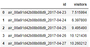
输出结果查看
sub.to_csv('result.csv', index=False)
import pandas as pd
df = pd.read_csv('result.csv')
df.head()


 1618
1618


 被折叠的 条评论
为什么被折叠?
被折叠的 条评论
为什么被折叠?
 到【灌水乐园】发言


