torch.nn

1. 参数

class torch.nn.Parameters

torch.nn.Parameter 是 torch.autograd.Variable 的子类，如果在网络的训练过程中需要更新，就要定义为Parameter, 类似为W(权重)和b(偏置)也都是Parameter。

Variable默认是不需要求梯度的，还需要手动设置参数 requires_grad=True，而且还不能作为model.parameters()中的参数直接送入优化器中，非常麻烦。

Pytorch主要通过引入nn.Parameter类型的变量和optimizer机制来解决了这个问题。Parameter是Variable的子类，本质上和后者一样，只不过parameter默认是求梯度的，同时一个网络中的parameter变量是可以通过 net.parameters() 来很方便地访问到的，只需将网络中所有需要训练更新的参数定义为Parameter类型，再用以optimizer，就能够完成所有参数的更新了，例如：optimizer = torch.optim.SGD(net.parameters(), lr=1e-1)。

请注意：net.parameters()中不包含我们在模型中定义的Variable，即使Variable设置了requires_grad=True。所以用Parameters方便很多。

2. 容器

class torch.nn.Module

Module类是所有神经网络模块的基类，我们的自定义模型也应该继承这个类。模块可以以树状结构包含其他的模块。Module类中包含网络层的定义以及forward方法，下面介绍如何定义一个网络：

1. 需要继承nn.Module类，并实现forward方法
2. 一般把网络中具有可学习参数的层放在构造函数__init__()中；
3. 不具有学习参数的层（如ReLU）可在forward中使用nn.functional来代替；
4. 只要在nn.Module的子类中定义了forward函数，利用Autograd自动实现反向求导。

import torch.nn as nn
import torch.nn.functional as F

class Model(nn.Module):
    def __init__(self):
        super(Model, self).__init__()
        # 添加子模块，也可以通过add_module来添加
        self.conv1 = nn.Conv2d(1,20,5)# submodule: Conv2d
        self.conv2 = nn.Conv2d(20,20,5)

    def forward(self,x):
        x = F.relu(self.conv1(x))
        return F.relu(self.conv2(x))

当调用.cuda()的时候，submodule（conv1和conv2）的参数也会转换为cuda Tensor。

方法：

• forward(* input)：定义了每次执行的 计算步骤。在所有的子类中都需要重写这个函数。

• train(mode=True)：将module设置为 training mode。仅仅当模型中有Dropout和BatchNorm是才会有影响。

• zero_grad()：将module中的所有模型参数的梯度设置为0，在反向传播之前的步骤。

• eval()：将模型设置成evaluation模式，仅仅当模型中有Dropout和BatchNorm时才会有影响。

• cpu(device_id=None)：将模型复制到CPU

• cuda(device_id=None)：将模型复制到GPU

• load_state_dict(state_dict)：加载模型参数，将state_dict中的parameters和buffers复制到此module和它的后代中。

• state_dict(destination=None, prefix=‘’)[source]：返回一个字典，保存着module的所有状态，包括parameters和buffers。

# 利用字典的items()函数打印模型的具体参数
model_dict = model.state_dict()
for k,v in model_dict.items():
    print(k)
    print(v)

• add_module(name, module)：将一个 child module 添加到当前 module。被添加的module可以通过 name属性来获取。 例如：

# 通过add_module添加子模型
self.add_module("conv",nn.Conv2d(10,20,4))

• children()：返回当前模型子模块的迭代器。可以利用该函数打印子模块，重复的子模块只被打印一次。

• modules()：返回一个包含 当前模型 所有模块的迭代器。重复的子模块只被打印一次。与children()不同的是，会打印模块本身及其子模块。

• named_children()：返回包含模型当前子模块的迭代器，yield 模块名字和模块本身。与上面的children不同，它还会返回子模块对应的name。

import torch.nn as nn
class Model(nn.Module):
    def __init__(self):
        super(Model, self).__init__()
        self.add_module("conv",nn.Conv2d(10,20,4))
        self.add_module("conv1",nn.Conv2d(20,10,4))
model = Model()
# 打印模块的名字的模块结构
for name, module in model.named_children():
    print(name)
    print(module)

结果：

conv
Conv2d(10, 20, kernel_size=(4, 4), stride=(1, 1))
conv1
Conv2d(20, 10, kernel_size=(4, 4), stride=(1, 1))

• named_modules(memo=None, prefix=‘’)[source]：返回包含网络中所有模块的迭代器, yielding 模块名和模块本身。

import torch.nn as nn
class Model(nn.Module):
    def __init__(self):
        super(Model, self).__init__()
        submodule = nn.Conv2d(10, 20, 4)
        self.add_module("conv", submodule)
        self.add_module("conv1", submodule)
model = Model()
# 循环打印这个模型的所有modules
for name, module in model.named_modules():
    print(name)
    print(module)

结果：

Model(
  (conv): Conv2d(10, 20, kernel_size=(4, 4), stride=(1, 1))
  (conv1): Conv2d(10, 20, kernel_size=(4, 4), stride=(1, 1))
)
conv
Conv2d(10, 20, kernel_size=(4, 4), stride=(1, 1))

• parameters(memo=None)：返回一个 包含模型所有参数 的迭代器。一般用来当作optimizer的参数。

• named_parameters(prefix=‘’, recurse=True)：返回一个遍历模块参数的迭代器，生成参数的名称和参数本身。

for name, param in self.named_parameters():
	if name in ['bias']:
		print(param.size())

• double()：将parameters和buffers的数据类型转换成double。

• float()：将parameters和buffers的数据类型转换成float。

• half()：将parameters和buffers的数据类型转换成half，half是半浮点数类型，即float16。

• apply(fn)：递归地将函数fn应用到父模块的每个子模块，也包括model这个父模块自身。

@torch.no_grad()
def init_weights(m):
    print(m)
    if type(m) == nn.Linear:
        m.weight.fill_(1.0)
        print(m.weight)
net = nn.Sequential(nn.Linear(2, 2), nn.Linear(2, 2))
net.apply(init_weights)

结果：

Linear(in_features=2, out_features=2, bias=True)
Parameter containing:
tensor([[1., 1.],
        [1., 1.]], requires_grad=True)
Linear(in_features=2, out_features=2, bias=True)
Parameter containing:
tensor([[1., 1.],
        [1., 1.]], requires_grad=True)
Sequential(
  (0): Linear(in_features=2, out_features=2, bias=True)
  (1): Linear(in_features=2, out_features=2, bias=True)
)

class torch.nn.Sequential(* args)

一个时序容器。Modules 会以他们传入的顺序被添加到容器中。用来创建子模块。

# Example of using Sequential

model = nn.Sequential(
          nn.Conv2d(1,20,5),
          nn.ReLU(),
          nn.Conv2d(20,64,5),
          nn.ReLU()
        )

class torch.nn.ModuleList(modules=None)[source]

将submodules保存在一个list中。

参数说明:

modules (list, optional) – 将要被添加到MuduleList中的 modules 列表

例子:

class MyModule(nn.Module):
    def __init__(self):
        super(MyModule, self).__init__()
        self.linears = nn.ModuleList([nn.Linear(10, 10) for i in range(10)])

    def forward(self, x):
        # ModuleList can act as an iterable, or be indexed         using ints
        for i, l in enumerate(self.linears):
            x = self.linears[i // 2](x) + l(x)
        return x

新增方法：

• append(module)：等价于 list 的 append()
  • module (nn.Module) – 要 append 的module
• extend(modules)：等价于 list 的 extend() 方法
  • modules (list) – list of modules to append

总结：创建子模块的方法：
（1）self.conv1 = nn.Conv2d(1,20,5)
（2）self.add_module(“conv”,nn.Conv2d(10,20,4))
（3）nn.Sequential( nn.Conv2d(1,20,5), nn.ReLU(), nn.Conv2d(20,64,5), nn.ReLU() )
（4）nn.ModuleList([nn.Linear(10, 10) for i in range(10)])，搭配append()和extend()使用

3. 卷积层

class torch.nn.Conv1d(in_channels, out_channels, kernel_size, stride=1, padding=0, dilation=1, groups=1, bias=True)

一维卷积层。

参数：

• groups(int, optional) – 控制输入和输出之间的连接，用于分组卷积和深度可分离卷积。
• bias(bool, optional) - 如果bias=True，添加偏置

形状：

• 输入: (N,C_in,L_in)
• 输出: (N,C_out,L_out)
• 输入输出的计算方式：

$$L_{out}=floor((L_{in}+2padding-dilation(kernerl\_size-1)-1)/stride+1)$$

class torch.nn.Conv2d(in_channels, out_channels, kernel_size, stride=1, padding=0, dilation=1, groups=1, bias=True)

二维卷积层。

class torch.nn.Conv3d(in_channels, out_channels, kernel_size, stride=1, padding=0, dilation=1, groups=1, bias=True)‘’

三维卷积层。

class torch.nn.ConvTranspose1d(in_channels, out_channels, kernel_size, stride=1, padding=0, output_padding=0, groups=1, bias=True)

一维反卷积。

参数：

• padding (int or tuple, optional)- 输入的每一条边补充0的层数
• output_padding(int or tuple, optional) - 输出的每一条边补充0的层数

形状：

• 输入: (N,C_in,L_in)
• 输出: (N,C_out,L_out)
• 输入输出的计算方式：

$$L_{out}=(L_{in}-1)stride-2padding+kernel\_size+output\_padding$$

class torch.nn.ConvTranspose2d(in_channels, out_channels, kernel_size, stride=1, padding=0, output_padding=0, groups=1, bias=True)

二维的反卷积。

torch.nn.ConvTranspose3d(in_channels, out_channels, kernel_size, stride=1, padding=0, output_padding=0, groups=1, bias=True)

三维的反卷积。

4. 池化层

class torch.nn.MaxPool1d(kernel_size, stride=None, padding=0, dilation=1, return_indices=False, ceil_mode=False)

1维最大池化。

参数：

• return_indices - 如果等于True，会返回输出最大值的序号，对于上采样操作会有帮助。用于upMaxPooling
• ceil_mode - 如果等于True，计算输出信号大小的时候，会使用向上取整，代替默认的向下取整的操作

形状:

• 输入: (N,C_in,L_in)
• 输出: (N,C_out,L_out)

$$L_{out}=floor((L_{in}+2padding-dilation(kernel\_size-1)-1)/stride+1)$$

class torch.nn.MaxPool2d(kernel_size, stride=None, padding=0, dilation=1, return_indices=False, ceil_mode=False)

2维最大池化。

class torch.nn.MaxPool3d(kernel_size, stride=None, padding=0, dilation=1, return_indices=False, ceil_mode=False)

3维最大池化。

class torch.nn.MaxUnpool1d(kernel_size, stride=None, padding=0)

Maxpool1d的逆过程，不过并不是完全的逆过程，因为在maxpool1d的过程中，一些最大值的已经丢失。 MaxUnpool1d输入MaxPool1d的输出，包括最大值的索引，并计算所有maxpool1d过程中非最大值被设置为零的部分的反向。

参数：

• kernel_size(int or tuple) - max pooling的窗口大小
• stride(int or tuple, optional) - max pooling的窗口移动的步长。默认值是kernel_size
• padding(int or tuple, optional) - 输入的每一条边补充0的层数

输入：

• input：需要转换的tensor
• indices：Maxpool1d的索引号
• output_size：一个指定输出大小的torch.Size

形状:

• input: (N,C,H_in)
• output:(N,C,H_out)

$$H_{out}=(H_{in}-1)stride[0]-2padding[0]+kernel\_size[0]$$
也可以使用output_size指定输出的大小

class torch.nn.MaxUnpool2d(kernel_size, stride=None, padding=0)

Maxpool2d的逆过程。

例子：

import torch
import torch.nn as nn
from torch.autograd import Variable

pool = nn.MaxPool2d(2, stride=2, return_indices=True)
unpool = nn.MaxUnpool2d(2,2)

input = Variable(torch.tensor([[[[1,2,3,4],
                                 [5,6,7,8],
                                 [9,10,11,12],
                                 [13,14,15,16]]]],dtype=torch.float32))

output,indices = pool(input)
print(output)

result = unpool(output,indices)
print(result)

result = unpool(output, indices, output_size=torch.Size([1, 1, 5, 5]))
print(result)

结果：

tensor([[[[ 6.,  8.],
          [14., 16.]]]])
tensor([[[[ 0.,  0.,  0.,  0.],
          [ 0.,  6.,  0.,  8.],
          [ 0.,  0.,  0.,  0.],
          [ 0., 14.,  0., 16.]]]])
tensor([[[[ 0.,  0.,  0.,  0.,  0.],
          [ 6.,  0.,  8.,  0.,  0.],
          [ 0.,  0.,  0., 14.,  0.],
          [16.,  0.,  0.,  0.,  0.],
          [ 0.,  0.,  0.,  0.,  0.]]]])

class torch.nn.MaxUnpool3d(kernel_size, stride=None, padding=0)

Maxpool3d的逆过程。

class torch.nn.AvgPool1d(kernel_size, stride=None, padding=0, ceil_mode=False, count_include_pad=True)

1维平均池化。

参数：

• ceil_mode - 如果等于True，计算输出信号大小的时候，会使用向上取整，代替默认的向下取整的操作
• count_include_pad - 如果等于True，计算平均池化时，将包括padding填充的0

形状：

• input:(N,C,L_in)
• output:(N,C,L_out)

$$L_{out}=floor((L_{in}+2\ast padding-kernel\_size)/stride+1)$$

class torch.nn.AvgPool2d(kernel_size, stride=None, padding=0, ceil_mode=False, count_include_pad=True)

2维平均池化。

class torch.nn.AvgPool3d(kernel_size, stride=None)

3维的平均池化.

class torch.nn.AdaptiveMaxPool1d(output_size, return_indices=False)

1维的自适应最大池化。

参数：

• output_size: 输出信号的尺寸
• return_indices: 如果设置为True，会返回输出的索引。对 nn.MaxUnpool1d有用，默认值是False

class torch.nn.AdaptiveMaxPool2d(output_size, return_indices=False)

例子：

import torch
import torch.nn as nn
from torch.autograd import Variable

m = nn.AdaptiveMaxPool2d((5,7))
input = Variable(torch.randn(1, 64, 8, 9))
output = m(input)
print(output.shape)

m = nn.AdaptiveMaxPool2d(7)
input = Variable(torch.randn(1, 64, 10, 9))
output = m(input)
print(output.shape)

结果：

torch.Size([1, 64, 5, 7])
torch.Size([1, 64, 7, 7])

class torch.nn.AdaptiveAvgPool1d(output_size)

1维的自适应平均池化.

class torch.nn.AdaptiveAvgPool2d(output_size)

2维的自适应平均池化.

5. 非线性激活

class torch.nn.ReLU(inplace=False)

对输入运用修正线性单元函数$ReLU(x)=max(0,x)$。

参数： inplace-选择是否进行覆盖运算

形状：

• 输入：$(N,\ast )$，星号代表任意数目附加维度
• 输出：$(N,\ast )$，与输入拥有同样的shape属性

class torch.nn.ReLU6(inplace=False)

对输入的每一个元素运用函数$ReLU6(x)=min(max(0,x),6)$，也就是限制输出的最大值为6，这是为了在一些内存受限的嵌入式设备上使用。

class torch.nn.ELU(alpha=1.0, inplace=False)

对输入的每一个元素运用函数$f(x)=max(0,x)+min(0,alpha\ast (e^x-1))$。

class torch.nn.PReLU(num_parameters=1, init=0.25)

对输入的每一个元素运用函数$PReLU(x)=max(0,x)+a\ast min(0,x)$，a是一个可学习参数。这是LeakyReLU的升级版。

注意：当为了表现更佳的模型而学习参数a时不要使用权重衰减（weight decay）

参数：

• num_parameters：需要学习的a的个数，默认等于1

• init：a的初始值，默认等于0.25

class torch.nn.LeakyReLU(negative_slope=0.01, inplace=False)

对输入的每一个元素运用$f(x)=max(0,x)+negative\_slope\ast min(0,x)$

参数：

• negative_slope：控制负斜率的角度，默认等于0.01
• inplace-选择是否进行覆盖运算

class torch.nn.Threshold(threshold, value, inplace=False)

Threshold定义：

$$y=x,ifx>=threshold$$
$$y=value,ifx<threshold$$

参数：

• threshold：阈值
• value：输入值小于阈值则会被value代替
• inplace：选择是否进行覆盖运算

class torch.nn.Sigmoid

对每个元素运用Sigmoid函数，Sigmoid 定义如下：

$$f(x)=1/(1+e^{-x})$$

class torch.nn.Tanh

对输入的每个元素，

$$f(x)=(e^x-e^{-x})/(e^x+e^{-x})$$

class torch.nn.LogSigmoid

对输入的每个元素，
$$LogSigmoid(x)=log(1/(1+e^{-x}))$$

class torch.nn.Softplus(beta=1, threshold=20)

对每个元素运用Softplus函数，Softplus 定义如下：

$$f(x)=(1/beta)\ast log(1+e^{(beta\ast xi)})$$

Softplus函数是ReLU函数的平滑逼近，Softplus函数可以使得输出值限定为正数。

为了保证数值稳定性，线性函数的转换可以使输出大于某个值。

参数：

• beta：Softplus函数的beta值

• threshold：阈值

class torch.nn.Softmax

对n维输入张量运用Softmax函数，将张量的每个元素缩放到（0,1）区间且和为1。

形状：

• 输入：(N, L)
• 输出：(N, L)

返回结果是一个与输入维度相同的张量，每个元素的取值范围在（0,1）区间。

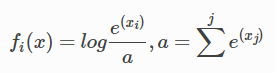
class torch.nn.LogSoftmax

对n维输入张量运用LogSoftmax函数，LogSoftmax函数定义如下：

形状：

• 输入：(N, L)
• 输出：(N, L)

6. 归一化层

class torch.nn.BatchNorm1d(num_features, eps=1e-05, momentum=0.1, affine=True)

对小批量(mini-batch)的2d或3d输入进行批标准化(Batch Normalization)操作

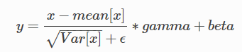
在每一个小批量（mini-batch）数据中，计算输入各个维度的均值和标准差。gamma与beta是可学习的大小为C的参数向量（C为输入大小）

在训练时，该层计算每次输入的均值与方差，并进行移动平均。移动平均默认的动量值为0.1。

在验证时，训练求得的均值/方差将用于标准化验证数据。

参数：

• num_features： 来自期望输入的特征数，该期望输入的大小为’batch_size x num_features [x width]’
• eps： 为保证数值稳定性（分母不能趋近或取0）,给分母加上的值。默认为1e-5。
• momentum： 动态均值和动态方差所使用的动量。默认为0.1。
• affine： 一个布尔值，当设为true，给该层添加可学习的仿射变换参数alpha和beta。

形状：

• 输入：（N, C）或者(N, C, L)
• 输出：（N, C）或者（N，C，L）（输入输出相同）

class torch.nn.BatchNorm2d(num_features, eps=1e-05, momentum=0.1, affine=True)

对小批量(mini-batch)3d数据组成的4d输入进行批标准化(Batch Normalization)操作

例子

input = Variable(torch.rand((20,100,35,45)))
# bn，学习仿射参数
bn = nn.BatchNorm2d(100)
output = bn(input)
print(output.shape)
# bn，不学习仿射参数
bn = nn.BatchNorm2d(100,affine=False)
output = bn(input)
print(output.shape)

结果：

torch.Size([20, 100, 35, 45])
torch.Size([20, 100, 35, 45])

class torch.nn.BatchNorm3d(num_features, eps=1e-05, momentum=0.1, affine=True)

对小批量(mini-batch)4d数据组成的5d输入进行批标准化(Batch Normalization)操作

7. 线性层

class torch.nn.Linear(in_features, out_features, bias=True)

对输入数据做线性变换：$y=Ax+b$

参数：

• in_features - 每个输入样本的大小
• out_features - 每个输出样本的大小
• bias - 若设置为False，这层不会学习偏置。默认值：True

形状：

• 输入: (N,in_features)
• 输出： (N,out_features)

变量：

• weight -形状为(out_features x in_features)的模块中可学习的权值
• bias -形状为(out_features)的模块中可学习的偏置

例子：

# 线性层
m = nn.Linear(20,30)
input = Variable(torch.rand((128,20)))
output = m(input)
print(output.size())

结果：

torch.Size([128, 30])

8. Dropout layers

class torch.nn.Dropout(p=0.5, inplace=False)

随机将输入张量中部分元素设置为0。对于每次前向调用，被置0的元素都是随机的。

参数：

• p - 将元素置0的概率。默认值：0.5
• in-place - 若设置为True，会在原地执行操作。默认值：False

形状：

• 输入： 任意。输入可以为任意形状。
• 输出： 相同。输出和输入形状相同。

例子：

m = nn.Dropout(p=0.2)
input = Variable(torch.rand((20,16))) # 批量一维输入
output = m(input)
print(output.shape)

input = Variable(torch.rand((3,32,20,16))) # 批量三维输入
output = m(input)
print(output.shape)

class torch.nn.Dropout2d(p=0.5, inplace=False)

随机将输入张量中整个通道设置为0。对于每次前向调用，被置0的通道都是随机的。通常输入来自Conv2d模块。

参数：

• p(float, optional) - 将元素置0的概率。
• in-place(bool, optional) - 若设置为True，会在原地执行操作。

形状：

• 输入： (N,C,H,W)
• 输出： (N,C,H,W)（与输入形状相同）

例子：

>>> m = nn.Dropout2d(p=0.2)
>>> input = autograd.Variable(torch.randn(20, 16, 32, 32))
>>> output = m(input)

class torch.nn.Dropout3d(p=0.5, inplace=False)

随机将输入张量中整个通道设置为0。对于每次前向调用，被置0的通道都是随机的。通常输入来自Conv3d模块。

参数：

• p(float, optional) - 将元素置0的概率。
• in-place(bool, optional) - 若设置为True，会在原地执行操作。

形状：

• 输入： N,C,D,H,W)
• 输出： (N,C,D,H,W)（与输入形状相同）

9. 损失函数

基本用法：

criterion = LossCriterion() #构造函数有自己的参数
loss = criterion(x, y) #调用标准时也有参数

计算出来的结果已经对mini-batch取了平均。

class torch.nn.L1Loss(size_average=True)

创建一个衡量输入x(模型预测输出)和目标y之间差的绝对值的平均值的标准。

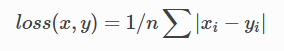
• x 和 y 可以是任意形状，每个包含n个元素。
• 对n个元素对应的差值的绝对值求和，得出来的结果除以n。
• 如果在创建L1Loss实例的时候在构造函数中传入size_average=False，那么求出来的绝对值的和将不会除以n

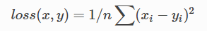
class torch.nn.MSELoss(size_average=True)

创建一个衡量输入x(模型预测输出)和目标y之间均方误差标准。

class torch.nn.CrossEntropyLoss(weight=None, size_average=True)

此标准将LogSoftMax和NLLLoss集成到一个类中。

当训练一个多类分类器的时候，这个方法是十分有用的。

• weight(tensor): 1-D tensor，n个元素，分别代表n类的权重，如果你的训练样本很不均衡的话，是非常有用的。默认值为None。

调用时参数：

• input : 包含每个类的得分，2-D tensor,shape为 batch*n

• target: 大小为 batch*n 的 2-D tensor，包含类别的索引(0到 n-1)。

Loss可以表述为以下形式：

当weight参数被指定的时候，loss的计算公式变为：

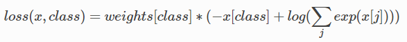
计算出的loss对mini-batch的大小取了平均。

class torch.nn.SmoothL1Loss(size_average=True)

平滑版L1 loss。

loss的公式如下：

此loss对于异常点的鲁棒性比MSELoss更强，而且，在某些情况下防止了梯度爆炸，(参照 Fast R-CNN)。这个loss有时也被称为 Huber loss。

x 和 y 可以是任何包含n个元素的tensor。默认情况下，求出来的loss会除以n。

class torch.nn.SoftMarginLoss(size_average=True)

创建一个标准，用来优化2分类的logistic loss。输入为 x（一个 2-D mini-batch Tensor）和 目标y（一个包含1或-1的Tensor）。

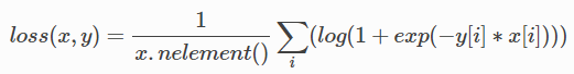
class torch.nn.MultiLabelSoftMarginLoss(weight=None, size_average=True)

创建一个标准，基于输入x和目标y的 max-entropy，优化多标签 one-versus-all 的损失。x:2-D mini-batch Tensor;y:binary 2D Tensor。对每个mini-batch中的样本，对应的loss为：

其中 I=x.nElement()-1, $y[i]\in 0,1$，y 和 x必须要有同样size。

10. 多GPU并行操作

torch.nn.DataParallel(module, device_ids=None, output_device=None, dim=0)

该容器通过在批处理维度中分组，将输入分割到指定的设备上，从而并行化给定模块的应用程序。在前向传播时，模块被复制到每个设备上，每个副本处理输入的一部分。在反向传播时，来自每个副本的梯度被累加到原始模块中。批处理大小应该大于所使用的GPU数量。

参数：

• module：我们定义的模型。
• device_ids：设备号列表。
• output_device：表示输出结果的设备。一般情况下是省略不写的，那么默认就是在device_ids[0]，也就是第一块卡上，也就解释了为什么第一块卡的显存会占用的比其他卡要更多一些。

例子：

device_ids = [0, 1] 	# id为0和1的两块显卡
model = torch.nn.DataParallel(model, device_ids=device_ids)
model = model.cuda() 

# 或者
device_ids = [0, 1]
model = torch.nn.DataParallel(model, device_ids=device_ids).cuda()

注：device_ids可以省略不写，根据源码，如果不写的时候，程序会自动帮你寻找可用的GPU设备。

11. 进阶

torch.nn.functional.unfold(input, kernel_size, dilation=1, padding=0, stride=1)

torch.nn.Fold(output_size, kernel_size, dilation=1, padding=0, stride=1)

官方的解释有点难懂，请移步https://blog.csdn.net/ViatorSun/article/details/119940759#