


目录
请注意:文章内容借鉴于Byzer官网,仅供参考。更多信息请访问Byzer官网(需保证外网访问速度)
一、Byzer-Python介绍
Byzer通过 Byzer-python 扩展(内置)来支持Python 代码。通过 Byzer-python,用户不仅仅可以进行使用 Python 进行 ETL 处理,比如可以将一个 Byzer 表转化成一个分布式DataFrame on Dask 来操作,支持各种机器学习框架,比如 Tensorflow,Sklearn,PyTorch。用户的Python脚本在 Byzer中是黑盒,用户可以通过固定API获得表数据,通过固定API来将Python输出转化为表,方便后续SQL处理。
下面看一个Hello Wrold的例子:
-- Byzer-python Hello World
select "world" as hello as table1;

!python conf "schema=st(field(hello,string))";
!python conf "pythonExec=/home/winubuntu/miniconda3/envs/byzerllm-desktop/bin/python";
!python conf "dataMode=model";
!python conf "runIn=driver";

run command as Ray.`` where
inputTable="table1"
and outputTable="new_table"
and code='''
import ray
from pyjava.api.mlsql import RayContext,PythonContext

ray_context = RayContext.connect(globals(),None)

rows_from_table1 = [item for item in ray_context.collect()]

for row in rows_from_table1:
   row["hello"] = "Byzer-Python"

context.build_result(rows_from_table1)
''';

select * from new_table as output;
简单描述下上面的代码。
第一步我们通过SQL获取到 table1
第二步我们设置一些配置参数
第三步我们通过 Ray 扩展来书写 Python 代码对 table1 里的每条记录做处理。
第四步我们把 Python处理的结果得到的表 new_table 进行输出。
当然,上面的hello world 代码无法处理大规模数据。我们在后续教程中会进行更详细的介绍。
二、Byzer-python工具语法糖
为了方便用户编写 Byzer-python 代码,我们在 Byzer-Notebook, Byzer Desktop 等产品中提供了如下的方式来写 Python代码:
#%python
#%input=command
#%output=test
#%schema=st(field(response,string))
#%runIn=driver
#%dataMode=model
#%cache=false
#%env=source /home/winubuntu/miniconda3/bin/activate byzerllm-desktop
#%pythonExec=/home/winubuntu/miniconda3/envs/byzerllm-desktop/bin/python

 import ray
from pyjava.api.mlsql import RayContext,PythonContext
from pyjava.storage import streaming_tar
from pyjava import rayfix
import os
import json
import logging
import sys

from byzerllm.moss.models.modeling_moss import MossForCausalLM
from byzerllm.moss.moss_inference import Inference

ray_context = RayContext.connect(globals(),"127.0.0.1:10001")

@ray.remote(num_gpus=1)
class Test():
    def __init__(self):
        pass

    def test(self):
        os.environ["CUDA_VISIBLE_DEVICES"] = "0"

        # Create an Inference instance with the specified model directory.
        print("init model")
        model = MossForCausalLM.from_pretrained("/home/winubuntu/projects/moss-model/moss-moon-003-sft-plugin-int4").half().cuda()
        print("infer")
        infer = Inference(model, device_map="auto")
        # Define a test case string.
        test_case = "<|Human|>: 你好 MOSS<eoh>\n<|MOSS|>:"

        # Generate a response using the Inference instance.
        res = infer(test_case)
        print(res)
        # Print the generated response.
        return res

res = ray.get(Test.remote().test.remote())
ray_context.build_result([{"response":res[0]}])
在上面代码中, 这些工具会提供语法糖,自动将 #% 注释 改写成 !python conf 设置,并且生成 run command as Ray 语法。此外,Byzer-Notebook 不需要自己手写这些注释,当你将Cell设置为 Python 代码时,会提供一个表格框方便你填写注释。注意:Byzer Notebook 暂时不能识别 pythonExec 参数,你需要使用 env 来设置。为了确保正确,你可以两个注释都填写上,就像上面的示例展示的那样。
三、环境依赖
在使用 Byzer-python 前,需要 Driver 的节点上配置好 Python 环境 ( Executor 节点可选) 。如果您使用 yarn 做集群管理,推荐使用 Conda 管理 Python 环境(参考Conda 环境安装)。而如果您使用 K8s,则可直接使用镜像管理。接下来,我们以 Conda 为例,介绍创建 Byzer-python 环境的流程。
1. Python 环境搭建
创建一个名字为 byzerllm-desktop 的 Python 3.10 环境
conda create -n byzerllm-desktop python=3.10
激活 byzerllm-desktop 环境
source activate byzerllm-desktop
安装基础以下基础依赖包
pandas==1.5.3
pyarrow==11.0.0
aiohttp==3.8.4
ray[default]==2.3.0
pyjava==0.5.0
2. Ray 环境搭建
Ray 是 Byzer 的运行时环境之一。尽管如此,他是可选的。当你有如下需求时:分布式Python处理,或者分布式 Pandas 的能力或者需要 GPU 等资源的管理能力,需要大模型等支持则用户需要部署 Ray 方便 Byzer 使用。Ray 依赖 Python 环境,需要和前面的环境保持一致。这里直接在 byzerllm-desktop 启动 Ray.
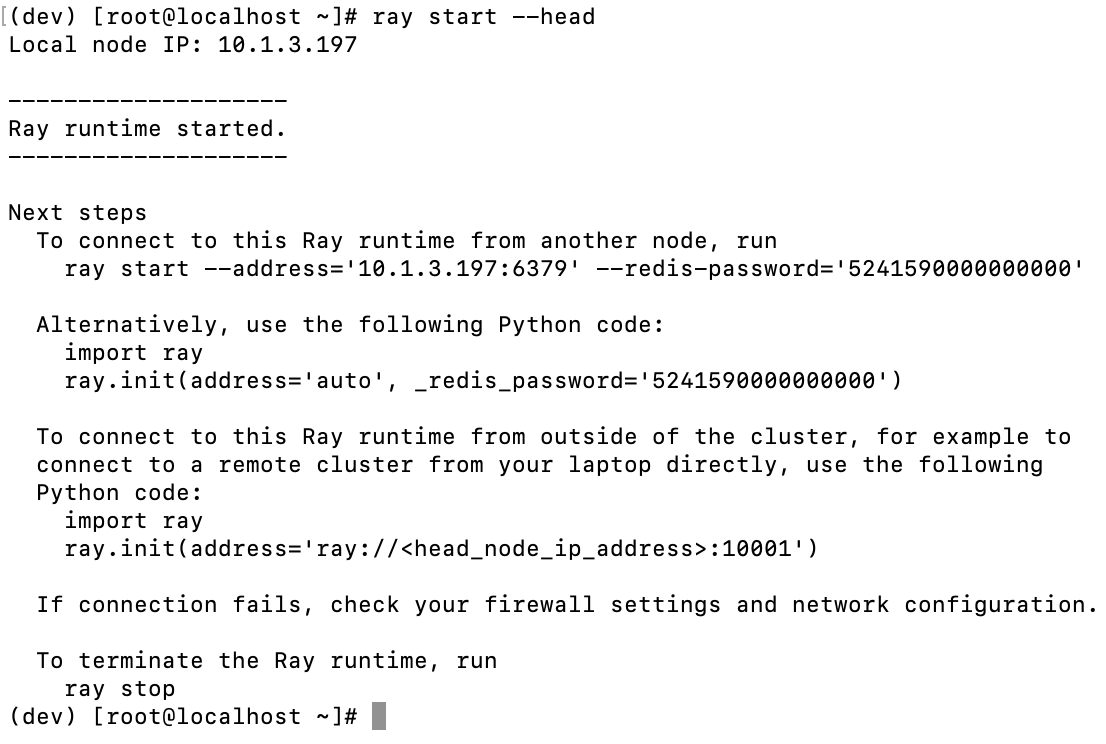
(1) 单机启动
ray start --head
看到以下日志说明启动成功:
运行上文日志中给出的 Python 代码,测试能否正常连接到 Ray 节点:
import ray
ray.init(address="ray://<head_node_ip_address>:10001") 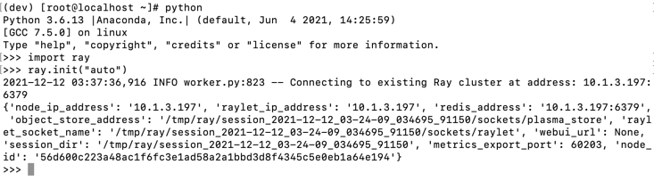
如果出现下方报错可能是 Conda 虚拟环境版本问题,建议重新安装

(2) 集群启动
在 Head 节点上运行
ray start --head
Worker 节点上运行
ray start --address='<head_node_ip_address>:6379' --redis-password='<password>'

下面是一个使用了Python高阶 API进行对SQL表进行分布式处理的一个示例。复制到 Byzer-Notebook中即可执行。
-- 分布式获取 python hello world

set jsonStr='''
{"Busn_A":114,"Busn_B":57},
{"Busn_A":55,"Busn_B":134},
{"Busn_A":27,"Busn_B":137},
{"Busn_A":101,"Busn_B":129},
{"Busn_A":125,"Busn_B":145},
{"Busn_A":27,"Busn_B":60},
{"Busn_A":105,"Busn_B":49}
''';

load jsonStr.`jsonStr` as data;

!python conf "pythonExec=/home/winubuntu/miniconda3/envs/byzerllm-desktop/bin/python";
!python conf "schema=st(field(ProductName,string),field(SubProduct,string))";
!python conf "dataMode=data";
!python conf "runIn=driver";

run command as Ray.`` where
inputTable="data"
and outputTable="python_output_table"
and code='''
from pyjava.api.mlsql import PythonContext,RayContext

# type hint
context:PythonContext = context

ray_context = RayContext.connect(globals(),"127.0.0.1:10001")

def echo(row):
    row1 = {}
    row1["ProductName"]=str(row['Busn_A'])+'_jackm'
    row1["SubProduct"] = str(row['Busn_B'])+'_product'
    return row1

ray_context.foreach(echo)
''';
3. Byzer-python 与 Ray
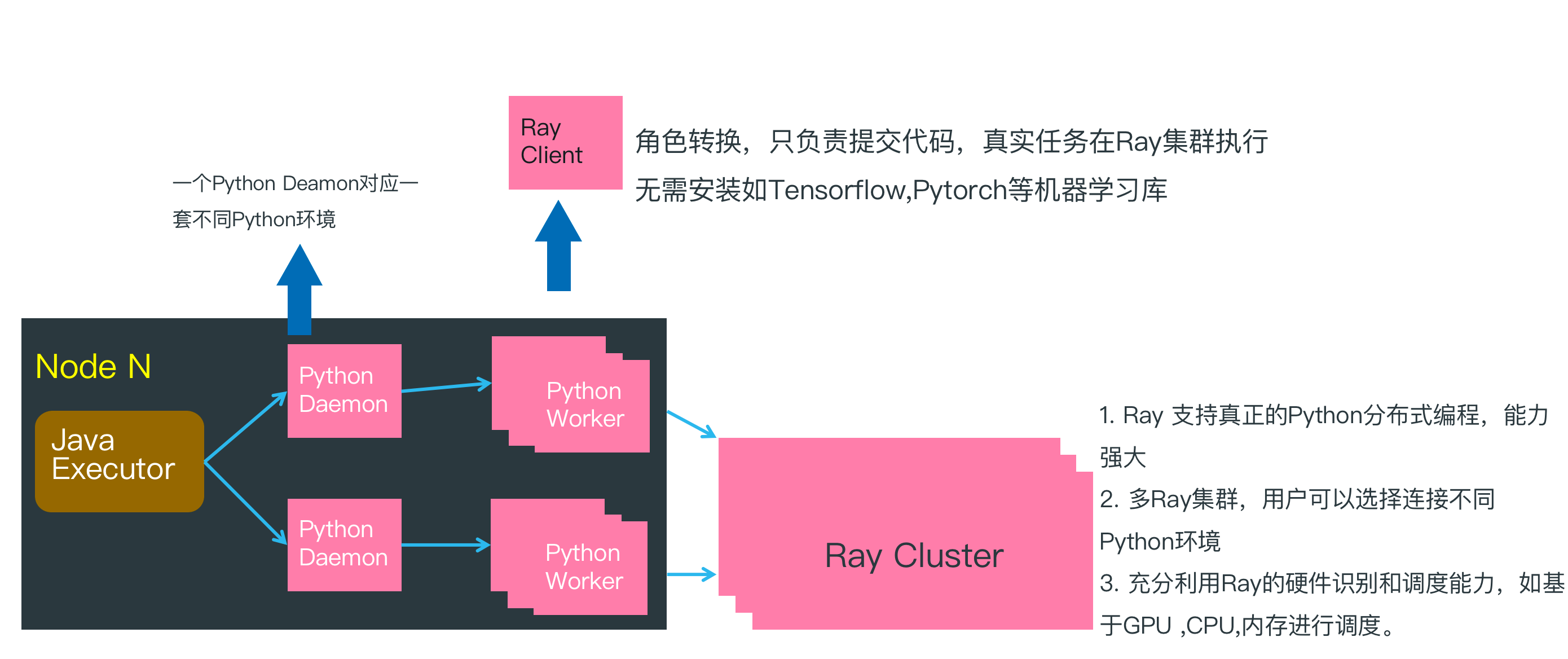
在上一篇 Hello World 例子中, 脚本在 Java Executor节点执行,然后再把 Byzer-python 代码传递给 Python Worker 执行。此时因为没有连接 Ray 集群,所以所有的逻辑处理工作都在 Python Worker 中完成,并且是单机执行。
在上文分布式的 Hello World 示例中, 通过连接 Ray Cluster, Python Worker 转化为 Ray Client,只负责把 Byzer-python 代码转化为任务提交给 Ray Cluster,所以在分布式计算场景下 Python Worker 可以很轻量,除了基本的 Ray,Pyjava 等库以外,不需要安装额外的 Python 依赖库。
四、参数详解
在前面的示例中,你会看到类似这样的配置:
!python conf "pythonExec=/home/winubuntu/miniconda3/envs/byzerllm-desktop/bin/python";
!python conf "schema=st(field(ProductName,string),field(SubProduct,string))";
!python conf "dataMode=data";
!python conf "runIn=driver";
这些配置决定了后续 Python 代码的执行模式。 比如 pythonExec 其实是指定 Python 代码在什么环境下执行。 schema 则决定了 Python的输出表的格式是什么。
(1)Byzer-python 常见参数:

(2)仅仅和模型部署相关的参数
|rayAddress| 设置一个 Ray 地址。 该参数对于部署模型有效| |num_gpus| 单个模型需要的GPU资源。该参数对于部署模型有效 | |maxConcurrency| 部署的模型需要支持的并发。该参数对于部署模型有效 | |standalone| 是不是只有一个模型节点。是的话设置为true,否则为false. 该参数对于部署模型有效 |
(3)Schema 表达
当我们使用 Python 代码创建新表输出的时候,需要手动指定 Schema. 有两种情况:
如果返回的是数据,可以通过设置 schema=st(field({name},{type})...) 定义各字段的字段名和字段类型;
如果返回到是文件,可设置 schema=file;
设置格式如下:
!python conf "schema=st(field(_id,string),field(x,double),field(y,double))";schema 字段类型对应关系:

此外,也支持 json/MySQL Create table 格式的设置方式.
json 格式符合 Spark 格式,你可以通过
!desc TableName json;
获取json格式示例。比如:
{"type":"struct",
 "fields":[
        {"name":"source","type":"string","nullable":true,"metadata":{}},
        {"name":"page_content","type":"string","nullable":true,"metadata":{}}
    ]
}
五、数据处理
在上一篇环境设置的里,我们提供了一个分布式做ETL处理的例子。等价于实现了一个 Python UDF(User-Defined-Function 用户自定义函数)。 在这一篇中,我们会详细介绍使用 Byzer-pyhton。
演示数据准备
set jsonStr='''
{"features":[5.1,3.5,1.4,0.2],"label":0.0},
{"features":[5.1,3.5,1.4,0.2],"label":1.0},
{"features":[5.1,3.5,1.4,0.2],"label":0.0},
{"features":[4.4,2.9,1.4,0.2],"label":0.0},
{"features":[5.1,3.5,1.4,0.2],"label":1.0},
{"features":[5.1,3.5,1.4,0.2],"label":0.0},
{"features":[5.1,3.5,1.4,0.2],"label":0.0},
{"features":[4.7,3.2,1.3,0.2],"label":1.0},
{"features":[5.1,3.5,1.4,0.2],"label":0.0},
{"features":[5.1,3.5,1.4,0.2],"label":0.0}
''';
load jsonStr.`jsonStr` as data;
保存至数据湖:
save overwrite data as delta.`example.mock_data`;
加载数据湖里的 mock_data,并做简单的处理,得到 sample_data。
load delta.`example.mock_data` as example_data;
select features[0] as a ,features[1] as b from example_data
as sample_data;
1. Byzer-python 处理数据
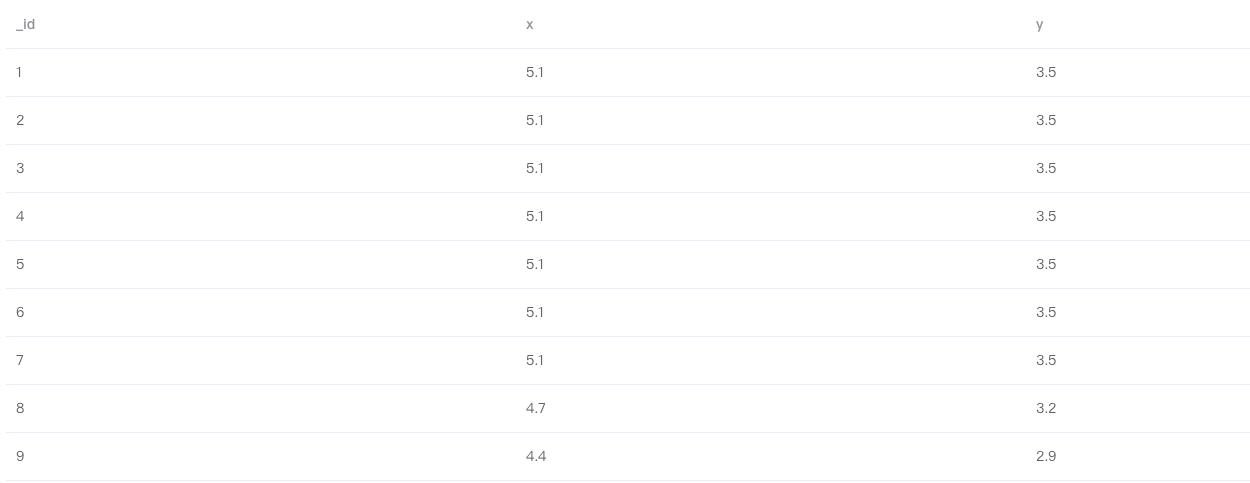
如果数据规模不大,可以在 Byzer-Notebook 中使用如下 Python 脚本对表 sample_data 进行处理:
#%python
#%input=sample_data
#%output=python_output_table
#%schema=st(field(_id,string),field(x,double),field(y,double))
#%runIn=driver
#%dataMode=model
#%cache=true
#%pythonExec=/home/winubuntu/miniconda3/envs/byzerllm-desktop/bin/python
#%env=source /home/winubuntu/miniconda3/bin/activate byzerllm-desktop

import ray
from pyjava.api.mlsql import RayContext

ray_context = RayContext.connect(globals(), None)
rows = RayContext.collect_from(ray_context.data_servers())
id_count = 1

def handle_record(row):
    global id_count
    item = {"_id": str(id_count)}
    id_count += 1
    item["x"] = row["a"]
    item["y"] = row["b"]
    return item

result = [handle_record(row) for row in rows]
context.build_result(result)
''';
上面的代码如果去Byzer-Notebook 提供的语法糖的话,会长成这个样子:
!python env "PYTHON_ENV=source /home/winubuntu/miniconda3/bin/activate byzerllm-desktop";
!python conf "runIn=driver"
!python conf "dataMode=model";
!python conf "schema=st(field(_id,string),field(x,double),field(y,double)

run command as Ray.`` where
inputTable="sample_data"
and outputTable="python_output_table"
and code='''
import ray
from pyjava.api.mlsql import RayContext

ray_context = RayContext.connect(globals(), None)
rows = RayContext.collect_from(ray_context.data_servers())
id_count = 1

def handle_record(row):
    global id_count
    item = {"_id": str(id_count)}
    id_count += 1
    item["x"] = row["a"]
    item["y"] = row["b"]
    return item

result = [handle_record(row) for row in rows]
context.build_result(result)
''';
2. Byzer-python 代码说明
注意到 Python 脚本以字符串参数形式出现在代码中,这是 Byzer-Python 代码的一个模版。其中参数 inputTable 指定需要处理的表,没有需要处理的表时,可设置为 command ;参数 outputTable 指定输出表的表名;参数 code 为需要执行的 Python 脚本。
run command as Ray.`` where
inputTable="sample_data"
and outputTable="python_output_table"
and code='''
import ray
......
''';
传入的 Python 脚本:
## 引入必要的包
import ray
from pyjava.api.mlsql import RayContext

## 获取 ray_context,如果需要使用 Ray 集群,那么第二个参数填写集群 Master 节点的地址
## 否则设置为None就好。
ray_context = RayContext.connect(globals(), None)

# 通过ray_context.data_servers() 获取所有数据源,如果开启了Ray,那么就可以
# 分布式获取这些数据进行处理。
rows = RayContext.collect_from(ray_context.data_servers())
id_count = 1

## 从 java 端接受的数据格式也是list(dict),也就是说,每一行的数据都以字典的数据结构存储。
## 比如 sample_data 的数据,在 Python 端拿到的结构就是
## [{'a':'5.1','b':'3.5'}, {'a':'5.1','b':'3.5'}, {'a':'5.1','b':'3.5'} ...]
## 基于这个数据结构,我们对输入数据进行数据处理
def handle_record(row):
    global id_count
    item = {"_id": str(id_count)}
    id_count += 1
    item["x"] = row["a"]
    item["y"] = row["b"]
    return item

result = [handle_record(row) for row in rows]

## 此处 result 是一个迭代器,context.build_result 也支持传入生成器/数组
context.build_result(result)
3. Byzer-python 读写 Excel 文件
Python 有很多处理 Excel 文件的库,功能成熟完善,您可以在 Byzer-python 环境中安装相应的库来处理您的 Excel 文件。这里以 pandas 为例来读取和保存 Excel 文件(需要安装 xlrd/xlwt 包,pip install xlrd==1.2.0 xlwt):
-- 将上文 sample_data 保存成 Excel 文件

!python env "PYTHON_ENV=source activate dev";
!python conf "schema=st(field(file,binary))";
!python conf "dataMode=model";
!python conf "runIn=driver";
run command as Ray.`` where
inputTable="sample_data"
and outputTable="excel_data"
and code='''
import io
import ray
import pandas as pd
from pyjava.api.mlsql import RayContext, PythonContext

ray_context = RayContext.connect(globals(), None)

data = ray_context.to_pandas()

output = io.BytesIO()
writer = pd.ExcelWriter(output, engine='xlwt')
data.to_excel(writer, index=False)
writer.save()
xlsx_data = output.getvalue()

context.build_result([{"file":xlsx_data}])
''';
!saveFile _ -i excel_data -o /tmp/sample_data.xlsx;
-- 读取 sample_data.xlsx 文件
load binaryFile.`/tmp/sample_data.xlsx` as excel_table;
!python env "PYTHON_ENV=source activate dev";
!python conf "schema=st(field(a,double),field(b,double))";
!python conf "dataMode=model";
!python conf "runIn=driver";
run command as Ray.`` where
inputTable="excel_table"
and outputTable="excel_data"
and code='''
import io
import ray
from pyjava.api.mlsql import RayContext
import pandas as pd
ray_context = RayContext.connect(globals(),None)
file_content = ray_context.to_pandas().loc[0, "content"]
df = pd.read_excel(io.BytesIO(file_content))
data = [row for row in df.to_dict('records')]
context.log_client.log_to_driver(data)
context.build_result(data)
''';4. Byzer-python 分布式计算
分布式处理依赖 Ray 环境,您可以参考Ray 环境搭建 搭建 Ray 集群。这里我们简单介绍下如何使用 Pyjava 高阶 API 使用 Ray 完成分布式计算:
!python env "PYTHON_ENV=source activate dev";
!python conf "schema=st(field(_id,string),field(x,double),field(y,double))";
!python conf "dataMode=model";
!python conf "runIn=driver";

run command as Ray.`` where
inputTable="sample_data"
and outputTable="python_output_table"
and code='''
import ray
from pyjava import rayfix
from pyjava.api.mlsql import RayContext
import socket

## 获取 ray_context,这里需要使用 Ray,第二个参数填写 Ray head-node 的地址和端口
ray_context = RayContext.connect(globals(), '127.0.0.1:10001')

## Ray 集群分布式处理
@ray.remote
@rayfix.last
def handle_record(servers):

    datas = RayContext.collect_from(servers)

    result = []
    for row in datas:
        item = {"_id": socket.gethostname()}
        item["x"] = row["a"]
        item["y"] = row["b"]
        result.append(item)
    return result

data_servers = ray_context.data_servers()
res =  ray.get(handle_record.remote(data_servers))
## 构造结果数据返回
context.build_result(res)
''';
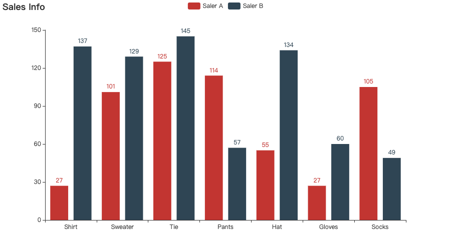
5. Byzer-python 图表绘制
您可以在 Byzer 桌面版 和 Bzyer Notebook 中使用 Python 绘图包(matplotlib、plotly、pyecharts 等,需要提前安装)绘制精美的图表,并用 Byzer-python 提供的 API 输出图片:
-- 绘图数据
set jsonStr='''
{"Busn_A":114,"Busn_B":57},
{"Busn_A":55,"Busn_B":134},
{"Busn_A":27,"Busn_B":137},
{"Busn_A":101,"Busn_B":129},
{"Busn_A":125,"Busn_B":145},
{"Busn_A":27,"Busn_B":60},
{"Busn_A":105,"Busn_B":49}
''';
load jsonStr.`jsonStr` as data;
使用 pyecharts 绘制图表:
!python env "PYTHON_ENV=source activate dev";
!python conf "schema=st(field(content,string),field(mime,string))";
!python conf "dataMode=model";
!python conf "runIn=driver";

run command as Ray.`` where
inputTable="data"
and outputTable="plt"
and code='''
from pyjava.api.mlsql import RayContext,PythonContext
from pyecharts import options as opts
import os
from pyecharts.charts import Bar

ray_context = RayContext.connect(globals(),None)

data = ray_context.to_pandas()
data_a = data['Busn_A']
data_b = data['Busn_B']

# 基本柱状图
bar = Bar()
bar.add_xaxis(["Shirt", "Sweater", "Tie", "Pants", "Hat", "Gloves", "Socks"])


bar.add_yaxis("Saler A", list(data_a))
bar.add_yaxis("Saler B", list(data_b))
bar.set_global_opts(title_opts=opts.TitleOpts(title="Sales Info"))
bar.render('bar_demo.html')  # 生成html文件
html = ""
with open("bar_demo.html") as file:
   html = "\n".join(file.readlines())
os.remove("bar_demo.html")
context.build_result([{"content":html,"mime":"html"}])
''';
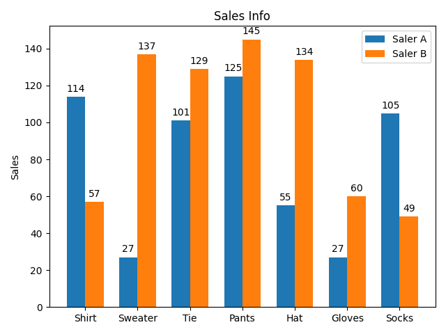
使用 matplotlib 绘制图表:
!python env "PYTHON_ENV=source activate dev";
!python conf "schema=st(field(content,string),field(mime,string))";
!python conf "dataMode=model";
!python conf "runIn=driver";

run command as Ray.`` where
inputTable="data"
and outputTable="plt"
and code='''
from pyjava.api.mlsql import RayContext,PythonContext
import matplotlib.pyplot as plt
import numpy as np
from pyjava.api import Utils
ray_context = RayContext.connect(globals(),None)

data = ray_context.to_pandas()


labels = ["Shirt", "Sweater", "Tie", "Pants", "Hat", "Gloves", "Socks"]
men_means = data['Busn_A']
women_means = data['Busn_B']

x = np.arange(len(labels))  # the label locations
width = 0.35  # the width of the bars

fig, ax = plt.subplots()
rects1 = ax.bar(x - width/2, men_means, width, label='Saler A')
rects2 = ax.bar(x + width/2, women_means, width, label='Saler B')

# Add some text for labels, title and custom x-axis tick labels, etc.
ax.set_ylabel('Sales')
ax.set_title('Sales Info')
ax.set_xticks(x)
ax.set_xticklabels(labels)
ax.legend()


def autolabel(rects):
    """Attach a text label above each bar in *rects*, displaying its height."""
    for rect in rects:
        height = rect.get_height()
        ax.annotate('{}'.format(height),
                    xy=(rect.get_x() + rect.get_width() / 2, height),
                    xytext=(0, 3),  # 3 points vertical offset
                    textcoords="offset points",
                    ha='center', va='bottom')


autolabel(rects1)
autolabel(rects2)

fig.tight_layout()

Utils.show_plt(plt, context)
''';
六、SQL表转化为分布式Pandas
运行本示例之前,需要安装dask:
pip install dask==2022.10.1
我们先通过 Byzer 语句加载一个数据集:
load csv.`/tmp/upload/iris-test.csv` where header="true" and inferSchema="true"
as iris;
接着我们在 Byzer-python中将该表转化为 分布式 Pandas API
#%python
#%input=iris
#%output=iris_scale1
#%schema=st(field(species,string),field(mean,double))
#%runIn=driver
#%dataMode=model
#%cache=true
#%pythonExec=/home/winubuntu/miniconda3/envs/byzerllm-desktop/bin/python
#%env=source /home/winubuntu/miniconda3/bin/activate byzerllm-desktop

from pyjava.api.mlsql import RayContext,PythonContext
import pandas as pd

context:PythonContext = context

ray_context = RayContext.connect(globals(),"127.0.0.1:10001")
# 把SQL表格数据转换为分布式 DataFrame
df = ray_context.to_dataset().to_dask()

print(df.head(10))

df2 = df.groupby("species").sepal_length.mean().compute()
df3 =  pd.DataFrame({"species":df2.index,"mean":df2.to_list()})

# 输出表格数据,供后续 SQL 使用
ray_context.build_result_from_dataframe(df3)
最后输出的结果可以继续在SQL中处理:
select * from iris_scale1 as output;七、模型训练
1. 单机训练
这里用到 tensorflow,运行前需要在 Driver 端安装
!python env "PYTHON_ENV=source activate dev";
!python conf "schema=st(field(epoch,string),field(k,string), field(b,string))";
!python conf "dataMode=model";
!python conf "runIn=driver";
run command as Ray.`` where
inputTable="command"
and outputTable="result"
and code='''
import ray
from pyjava import rayfix
from pyjava.api.mlsql import RayContext,PythonContext
# import tensorflow as tf
ray_context = RayContext.connect(globals(), None)
# 上面导包找不到placeholder模块时,换下面导入方式
import tensorflow.compat.v1 as tf
tf.disable_v2_behavior()
import numpy as np # Python的一种开源的数值计算扩展
import matplotlib.pyplot as plt # Python的一种绘图库
np.random.seed(5) # 设置产生伪随机数的类型
sx = np.linspace(-1, 1, 100) # 在-1到1之间产生100个等差数列作为图像的横坐标
# 根据y=2*x+1+噪声产生纵坐标
# randn(100)表示从100个样本的标准正态分布中返回一个样本值,0.4为数据抖动幅度
sy = 2 * sx + 1.0 + np.random.randn(100) * 0.4
def model(x, k, b):
return tf.multiply(k, x) + b
def train():
# 定义模型中的参数变量,并为其赋初值
k = tf.Variable(1.0, dtype=tf.float32, name='k')
b = tf.Variable(0, dtype=tf.float32, name='b')
# 定义训练数据的占位符,x为特征值,y为标签
x = tf.placeholder(dtype=tf.float32, name='x')
y = tf.placeholder(dtype=tf.float32, name='y')
# 通过模型得出特征值x对应的预测值yp
yp = model(x, k, b)
# 训练模型,设置训练参数(迭代次数、学习率)
train_epoch = 10
rate = 0.05
# 定义均方差为损失函数
loss = tf.reduce_mean(tf.square(y - yp))
# 定义梯度下降优化器,并传入参数学习率和损失函数
optimizer = tf.train.GradientDescentOptimizer(rate).minimize(loss)
ss = tf.Session()
init = tf.global_variables_initializer()
ss.run(init)
res = []
# 进行多轮迭代训练,每轮将样本值逐个输入模型,进行梯度下降优化操作得出参数,绘制模型曲线
for _ in range(train_epoch):
for x1, y1 in zip(sx, sy):
ss.run([optimizer, loss], feed_dict={x: x1, y: y1})
tmp_k = k.eval(session=ss)
tmp_b = b.eval(session=ss)
res.append((str(_), str(tmp_k), str(tmp_b)))
return res
res = train()
res = [{'epoch':item[0], 'k':item[1], 'b':item[2]} for item in res]
context.build_result(res)
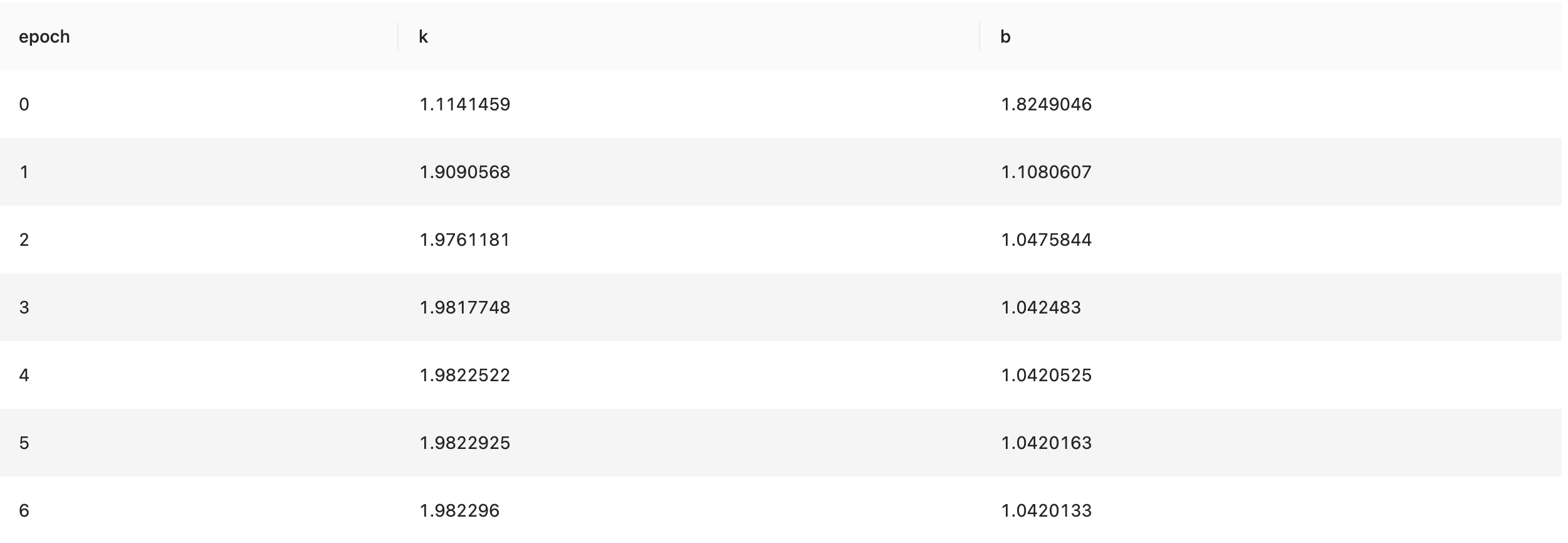
''';结果展示了每一个 epoch 的斜率(k)和截距(b)的拟合数据
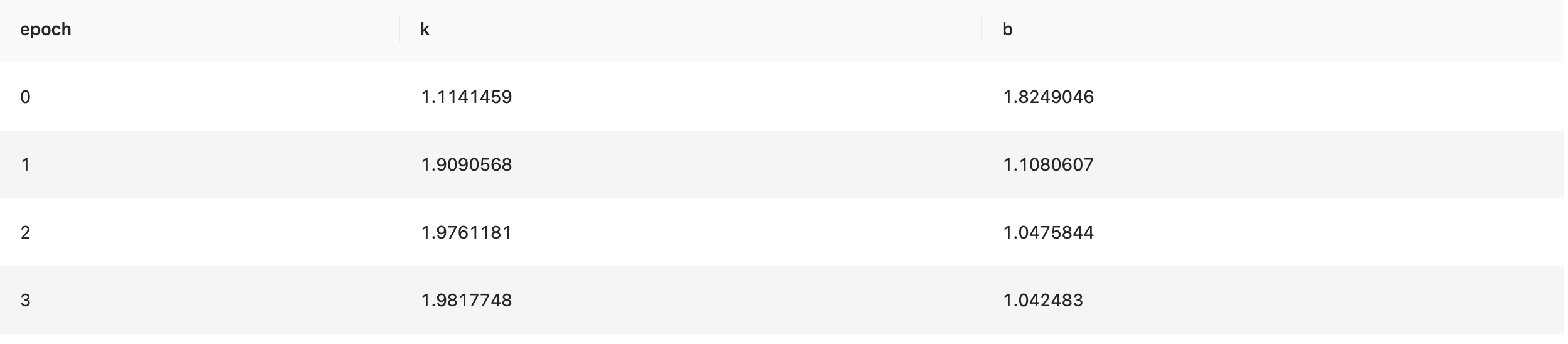
2. 分布式训练
运行前需要在 Ray 环境中安装 tensorflow
!python env "PYTHON_ENV=source activate dev";
!python conf "schema=st(field(epoch,string),field(k,string), field(b,string))";
!python conf "dataMode=model";
!python conf "runIn=driver";

run command as Ray.`` where
inputTable="command"
and outputTable="result"
and code='''
import ray
from pyjava import rayfix
from pyjava.api.mlsql import RayContext,PythonContext
# import tensorflow as tf
ray_context = RayContext.connect(globals(), url="127.0.0.1:10001")

@ray.remote
@rayfix.last
def train(servers):
    # 上面导包找不到placeholder模块时,换下面导入方式
    import numpy as np  # Python的一种开源的数值计算扩展
    import matplotlib.pyplot as plt  # Python的一种绘图库
    import tensorflow.compat.v1 as tf
    tf.disable_v2_behavior()
    np.random.seed(5)  # 设置产生伪随机数的类型
    sx = np.linspace(-1, 1, 100)  # 在-1到1之间产生100个等差数列作为图像的横坐标
    # 根据y=2*x+1+噪声产生纵坐标
    # randn(100)表示从100个样本的标准正态分布中返回一个样本值,0.4为数据抖动幅度
    sy = 2 * sx + 1.0 + np.random.randn(100) * 0.4
    # 定义模型中的参数变量,并为其赋初值
    k = tf.Variable(1.0, dtype=tf.float32, name='k')
    b = tf.Variable(0, dtype=tf.float32, name='b')
    # 定义训练数据的占位符,x为特征值,y为标签
    x = tf.placeholder(dtype=tf.float32, name='x')
    y = tf.placeholder(dtype=tf.float32, name='y')
    # 通过模型得出特征值x对应的预测值yp
    yp = tf.multiply(k, x) + b
    # 训练模型,设置训练参数(迭代次数、学习率)
    train_epoch = 10
    rate = 0.05
    # 定义均方差为损失函数
    loss = tf.reduce_mean(tf.square(y - yp))
    # 定义梯度下降优化器,并传入参数学习率和损失函数
    optimizer = tf.train.GradientDescentOptimizer(rate).minimize(loss)
    ss = tf.Session()
    init = tf.global_variables_initializer()
    ss.run(init)
    res = []
    # 进行多轮迭代训练,每轮将样本值逐个输入模型,进行梯度下降优化操作得出参数,绘制模型曲线
    for _ in range(train_epoch):
        for x1, y1 in zip(sx, sy):
            ss.run([optimizer, loss], feed_dict={x: x1, y: y1})
        tmp_k = k.eval(session=ss)
        tmp_b = b.eval(session=ss)
        res.append((str(_), str(tmp_k), str(tmp_b)))
    return res


data_servers = ray_context.data_servers()
res =  ray.get(train.remote(data_servers))
res = [{'epoch':item[0], 'k':item[1], 'b':item[2]} for item in res]
context.build_result(res)
''';
八、模型部署
在 Byzer 中,我们可以使用和内置算法一样的方式将一个基于 Byzer-python 训练出的 AI 模型注册成一个 UDF 函数,这样可以将模型应用于批、流,以及 Web 服务中。接下来我们将展示 Byzer-python 基于 Ray 从模型训练再到模型部署的全流程 demo。
1. 数据准备
首先,安装 tensorflow 和 keras:
pip install keras tensorflow "tenacity~=6.2.0"准备 mnist 数据集(需要):
!python env "PYTHON_ENV=source activate ray1.8.0";
!python conf "schema=st(field(image,array(long)),field(label,long),field(tag,string))";
!python conf "runIn=driver";
!python conf "dataMode=model";

run command as Ray.`` where
inputTable="command"
and outputTable="mnist_data"
and code='''
from pyjava.api.mlsql import RayContext, PythonContext
from keras.datasets import mnist

ray_context = RayContext.connect(globals(), None)

(x_train, y_train),(x_test, y_test) = mnist.load_data()

train_images = x_train.reshape((x_train.shape[0], 28 * 28))
test_images = x_test.reshape((x_test.shape[0], 28 * 28))

train_data = [{"image": image.tolist(), "label": int(label), "tag": "train"} for (image, label) in zip(train_images, y_train)]
test_data = [{"image": image.tolist(), "label": int(label), "tag": "test"} for (image, label) in zip(test_images, y_test)]
context.build_result(train_data + test_data)
''';

save overwrite mnist_data as delta.`ai_datasets.mnist`;
上面的 Byzer-python 脚本,获取keras自带的 mnist 数据集,再将数据集保存到数据湖中。
2. 训练模型
接着就开始拿测试数据 minist 进行训练,下面是模型训练代码:
-- 获取训练数据集
load delta.`ai_datasets.mnist` as mnist_data;
select image, label from mnist_data where tag="train" as mnist_train_data;

!python env "PYTHON_ENV=source activate ray1.8.0";
!python conf "schema=file";
!python conf "dataMode=model";
!python conf "runIn=driver";

run command as Ray.`` where
inputTable="mnist_train_data"
and outputTable="mnist_model"
and code='''
import ray
import os
import tensorflow as tf
from pyjava.api.mlsql import RayContext
from pyjava.storage import streaming_tar
import numpy as np


ray_context = RayContext.connect(globals(),"127.0.0.1:10001")
data_servers = ray_context.data_servers()

train_dataset = [item for item in RayContext.collect_from(data_servers)]

x_train = np.array([np.array(item["image"]) for item in train_dataset])
y_train = np.array([item["label"] for item in train_dataset])

x_train = x_train.reshape((len(x_train),28, 28))

model = tf.keras.models.Sequential([
  tf.keras.layers.Flatten(input_shape=(28, 28)),
  tf.keras.layers.Dense(128, activation='relu'),
  tf.keras.layers.Dropout(0.2),
  tf.keras.layers.Dense(10, activation='softmax')
])

model.compile(optimizer='adam',
              loss='sparse_categorical_crossentropy',
              metrics=['accuracy'])

model.fit(x_train, y_train, epochs=5)

model_path = os.path.join("tmp","minist_model")
model.save(model_path)
model_binary = [item for item in streaming_tar.build_rows_from_file(model_path)]

ray_context.build_result(model_binary)
''';
最后把模型保存至数据湖里:
save overwrite mnist_model as delta.`ai_model.mnist_model`;3. 将模型注册成 UDF 函数
训练好模型之后,我们就可以用 Byzer-lang 的 Register 语法将模型注册成基于 Ray 的服务了,下面是模型注册的代码:
!python env "PYTHON_ENV=source activate ray1.8.0";
!python conf "schema=st(field(content,string))";
!python conf "mode=model";
!python conf "runIn=driver";
!python conf "rayAddress=127.0.0.1:10001";


-- 加载前面训练好的tf模型
load delta.`ai_model.mnist_model` as mnist_model;

-- 把模型注册成udf函数
register Ray.`mnist_model` as model_predict where
maxConcurrency="8"
and debugMode="true"
and registerCode='''

import ray
import numpy as np
from pyjava.api.mlsql import RayContext
from pyjava.udf import UDFMaster,UDFWorker,UDFBuilder,UDFBuildInFunc

ray_context = RayContext.connect(globals(), context.conf["rayAddress"])

# 预测函数
def predict_func(model,v):
    test_images = np.array([v])
    predictions = model.predict(test_images.reshape((1,28*28)))
    return {"value":[[float(np.argmax(item)) for item in predictions]]}

# 将预测函数提交到 ray_context
UDFBuilder.build(ray_context,UDFBuildInFunc.init_tf,predict_func)

''' and
predictCode='''

import ray
from pyjava.api.mlsql import RayContext
from pyjava.udf import UDFMaster,UDFWorker,UDFBuilder,UDFBuildInFunc

ray_context = RayContext.connect(globals(), context.conf["rayAddress"])

#
UDFBuilder.apply(ray_context)

''';
这里 UDFBuilder 与 UDFBuildInFunc 都是 Pyjava 提供的高阶 API,用来将 Python 脚本注册成 UDF 函数。
4. 使用模型做预测
Byzer 提供了类 SQL 语句做批量(Batch)查询,加载您的数据集,即可对数据进行预测。
load delta.`ai_datasets.mnist` as mnist_data;
select cast(image as array<double>) as image, label as label from mnist_data where tag = "test" limit 100 as mnist_test_data;
select model_predict(array(image))[0][0] as predicted, label as label  from  mnist_test_data as output;
后续可以直接调用 Byzer-engine 的 Rest API, 使用注册好的 UDF 函数对您的数据集作预测。
九、PyJava API简介
前面的示例中,可以看到类似 RayContext、 PythonContext 这些对象。这些对象帮助用户进行输入和输出的控制。
Byzer-python 代码编写三步走:
1. 初始化 RayContext
ray_context = RayContext.connect(globals(), "192.168.1.7:10001")其中第二个参数是可选的,用来设置 Ray 集群 Master 节点地址和端口。如果不需要连接 Ray 集群,则设置为 None 即可。
2. 获取数据
获取所有数据:
# 获取 DataFrame
data = ray_context.to_pandas()

# 获取一个返回值为 dict 类型的生成器
items = ray_context.collect()注意,ray_context.collect() 得到的生成器只能迭代一次。
通过分片来获取数据:
data_refs = ray_context.data_servers()

data = [RayContext.collect_from([data_ref]) for data_ref in data_refs]注意,data_refs 是字符串数组,每个元素是一个 ip:port 的形态. 可以使用 RayContext.collect_from 单独获取每个数据分片。
如果数据规模大,可以转化为 Dask 数据集来进行操作:
data = ray_context.to_dataset().to_dask()3. 构建新的结果数据输出
context.build_result(data) 这里 PythonContext.build_result 的入参 data 是可迭代对象,支持数组、生成器等
现在引入下面两个 API 用来做数据分布式处理:
(1)RayContext.foreach
如果已经连接了 Ray,那么可以直接使用高阶 API RayContext.foreach
set jsonStr='''

{"Busn_A":114,"Busn_B":57},

{"Busn_A":55,"Busn_B":134},

{"Busn_A":27,"Busn_B":137},

{"Busn_A":101,"Busn_B":129},

{"Busn_A":125,"Busn_B":145},

{"Busn_A":27,"Busn_B":60},

{"Busn_A":105,"Busn_B":49}

''';

load jsonStr.`jsonStr` as data;

!python env "PYTHON_ENV=source activate dev";
!python conf "schema=st(field(ProductName,string),field(SubProduct,string))";
!python conf "dataMode=data";
!python conf "runIn=driver";

run command as Ray.`` where
inputTable="data"
and outputTable="data2"
and code='''
import ray
from pyjava.api.mlsql import RayContext,PythonContext

context:PythonContext = context
ray_context = RayContext.connect(globals(),"127.0.0.1:10001")

def echo(row):
    row1 = {}
    row1["ProductName"]=str(row['a'])+'_jackm'
    row1["SubProduct"] = str(row['b'])+'_product'
    return row1
buffer = ray_context.foreach(echo)
''';
RayContext.foreach 接收一个回调函数,函数的入参是单条记录。无需显示的申明如何获取数据,只要实现回调函数即可。
(2)RayContext.map_iter
我们也可以获得一批数据,可以使用 RayContext.map_iter。
系统会自动调度多个任务到 Ray 上并行运行。 map_iter 会根据表的分片大小启动相应个数的 task,如果你希望通过 map_iter 拿到所有的数据,而非部分数据,可以先对表做重新分区:
!python env "PYTHON_ENV=source activate dev";
!python conf "schema=st(field(ProductName,string),field(SubProduct,string))";
!python conf "dataMode=data";
!python conf "runIn=driver";

run command as Ray.`` where
inputTable="data"
and outputTable="data2"
and code='''
import ray
from pyjava.api.mlsql import RayContext
import numpy as np;
import time
ray_context = RayContext.connect(globals(),"127.0.0.1:10001")

def echo(rows):
    count = 0
    for row in rows:
      row1 = {}
      row1["ProductName"]="jackm"
      row1["SubProduct"] = str(row["Busn_A"])+'_'+str(row["Busn_B"])
      count = count + 1
      if count%1000 == 0:
          print("=====> " + str(time.time()) + " ====>" + str(count))
      yield row1

ray_context.map_iter(echo)
''';
(3)将表转化为分布式 DataFrame
如果用户喜欢使用 Pandas API,而数据集又特别大,也可以将数据转换为分布式 DataFrame on Dask 来做进一步处理:
!python env "PYTHON_ENV=source activate dev";
!python conf "schema=st(field(count,long))";
!python conf "dataMode=model";
!python conf "runIn=driver";

run command as Ray.`` where
inputTable="data"
and outputTable="data2"
and code='''
from pyjava.api.mlsql import PythonContext,RayContext
context:PythonContext = context

ray_context = RayContext.connect(globals(),"127.0.0.1:10001")
df = ray_context.to_dataset().to_dask()
c = df.shape[0].compute()
context.build_result([{"count":c}])
''';- 使用该 API 需要连接到 Ray,需要配置节点地址。
- 对应的 Python 环境需要预先安装好 dask ,
pip install "dask[complete]"
(4)将目录转化为表
这个功能在做算法训练的时候特别有用。比如模型训练完毕后,一般是保存在训练所在的节点上的。我们需要将其转化为表,并且保存到数据湖里去。具体操作如下:
首先,通过 Byzer-python 读取目录,转化为表:
!python env "PYTHON_ENV=source activate dev";
!python conf "schema=file";
!python conf "dataMode=model";
!python conf "runIn=driver";


run command as Ray.`` where
inputTable="train_data"
and outputTable="model_output"
and code='''
import os
from pyjava.storage import streaming_tar
from pyjava.api.mlsql import PythonContext,RayContext

context:PythonContext = context
ray_context = RayContext.connect(globals(), None)

# train your model here
......

model_path = os.path.join("/","tmp","ai_model/model")
your_model.save(model_path)

model_binary = [item for item in streaming_tar.build_rows_from_file(model_path)]

context.build_result(model_binary)
''';
将 Byzer-python 产生的表保存到数据湖里
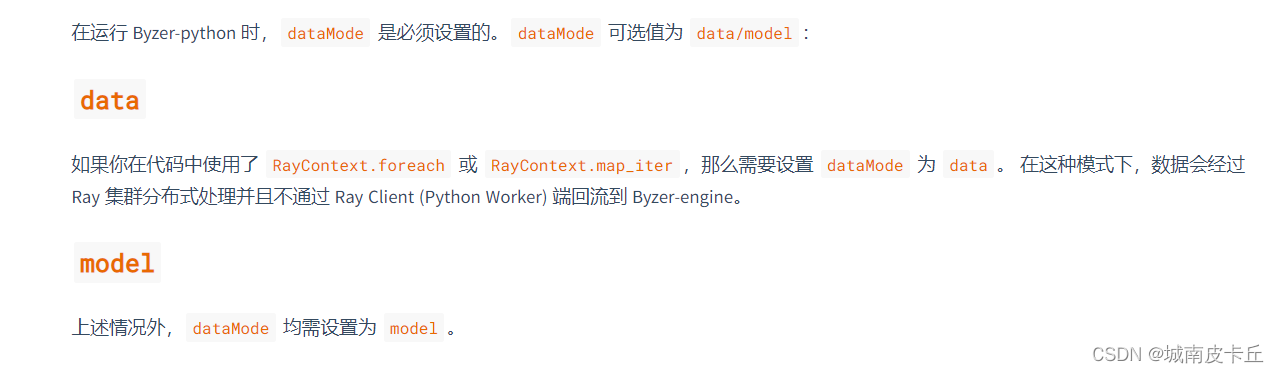
save overwrite model_output as delta.`ai_model.model_output`;十、dataMode 详解


 430
430


 被折叠的 条评论
为什么被折叠?
被折叠的 条评论
为什么被折叠?
 到【灌水乐园】发言


