Regression is All you Need

Regression is All you Need

Author: Bobby(Zhuoran) Peng

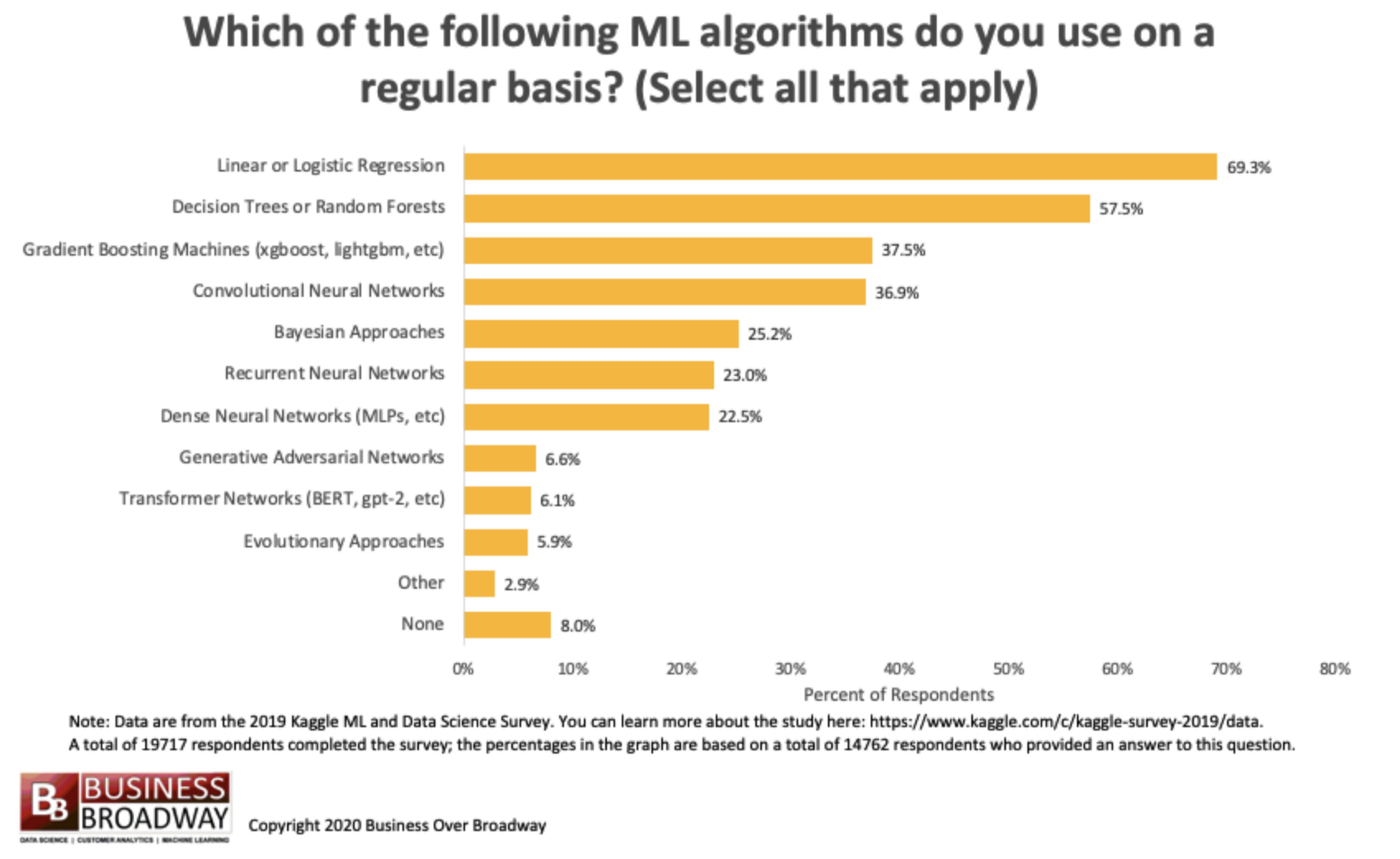
People have created and utilized a bewildering variety of algorithms trying to predict future data in various industries. However, the most prevalent and perhaps east-to-intrpret and proven algorithm remains to be linear regression. The following figure showing linear regression to be the most welcomed algorithm also implies that it is one of the most basic rules for supervised machine learning and beyond.

What is Linear Regression

There are two variables in a linear regression, one is dependent variable and the other is independent variable. The dependent variable is what we want to predict, and its value depends on the changes of independent variable.
$$y={\alpha }_0+{\alpha }_{1}x$$
In the above model, we are using x to predict the value of y.

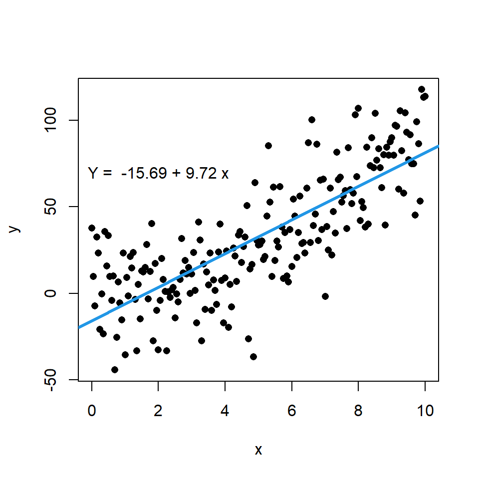
The above scatter plot is an example of a linear regression model. Here we get a fitting line of $y=-15.69+9.72x$, if we then have a $x$ value, we can use the equation to predict a $y$ value.

Also, we can use matrix to present the linear relationship. Let $X$ be a $d\times n$ matrix ($n$ items and $d$ features), and $w$ be $d\times 1$ matrix (containing cooeficients), and $\bar{Y}$ be the output matrix of size $n\times 1$, then we have: $$X^{T}w=\bar{Y}$$

Data in the real world are just like this scatter plot, our linear regression model is just a prediction, and we use $\bar{y}$ to present the predicted values of the model on our blue fitting line, while real data are those black spots scattering in the figure. The difference between the predicted $\bar{y}$ and the real $y$ value is called the error, and we often use $e$ to represent it, and we have the following equation: $$y={\alpha }_0+{\alpha }_{1}x+e$$ or $$Y=X^{T}w+e$$

The Error Function

As mentioned above, error is the distance between $y$ and $\bar{y}$, then we can derive a way to estimate the total error of the whole set: $$E=\sum _{i=1}^n(y_i-\overline{y_i}{)}^2=\sum _{i=1}^n(y_i-{\alpha }_0-{\alpha }_1{x}_i{)}^2$$ or $$E=||Y-X^{T}w|{|}^2$$And this is obviously a quadratic function. Thus to minimize the error, we need to manipulate ${\alpha }_0$ and ${\alpha }_1$, or $w$ matrice, taking derivative until it reaches 0. Thus we have: $$\frac{\partial E}{\partial {\alpha }_0}=2\sum _{i=1}^n(y_i-{\alpha }_0-{\alpha }_1{x}_i)=0$$ $$\frac{\partial E}{\partial {\alpha }_1}=2\sum _{i=1}^n(y_i-{\alpha }_0-{\alpha }_1{x}_i)x_i=0$$
or for the matrix expression:$$\begin{gathered} E=||Y-X^{T}w|{|}^2=(Y-X^{T}w{)}^T(Y-X^{T}w) \\ =w^{T}X{X}^{T}w-w^{T}XY-Y^T{X}^{T}w+Y^{T}Y \end{gathered}$$
Then $$\begin{gathered} \frac{\partial E}{\partial w}=2X{X}^{T}w-2XY=0 \\ w=(X{X}^T{)}^{-1}Y \end{gathered}$$

Correlation is not Causality

We now know how to analyze a linear regression to predict y by x. In real life practices, two variables may have a strong correlation in the linear model, but this does not necessaryly mean x is the cause of y. For example, in a searching engine, items of higher ranking would recieve higher click rates, like the following figure showing.

You may find a linear relation between ranking and click rates, but this does not lead to the conclusion that users like items of higher ranking more than items of lower ranking. This is the typical position bias in recommender system, and the causality inspired machine learning problems are getting increasing focus these days, trying to find real causes behind linear or nonlinear correlations.