Amdahl‘s Law+ Gustafson-Barsis‘s Law

Amdahl’s Law

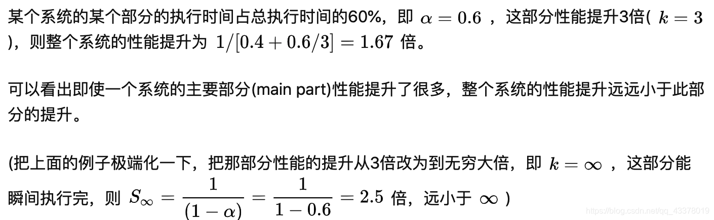
If 95% of the program can be parallelized, the theoretical maximum
speedup using parallel computing would be 20×, no matter how
many processors are used, i.e. if the non-parallelisable part takes 1
hour, then no matter how many cores you throw at it, it won’t
complete in <1 hour.

Consider a program that executes a single loop, where all
iterations can be computed independently, i.e., code can be
parallelized. By splitting the loop into several parts, e.g., one loop
iteration per processor, each processor now has to deal with loop
overheads such as calculation of bounds, test for loop completion
etc. This overhead is replicated as many times as there are
processors. In effect, loop overhead acts as a further (serial)
overhead in running the code. Also getting data to/from many
processor overheads?
In a nutshell Amdahl’s Law greatly simplifies the real world!
It also assumes a fixed problem size – sometimes can’t predict
length of time required for jobs,
– e.g., state space exploration or differential equations that don’t solve…

举例：

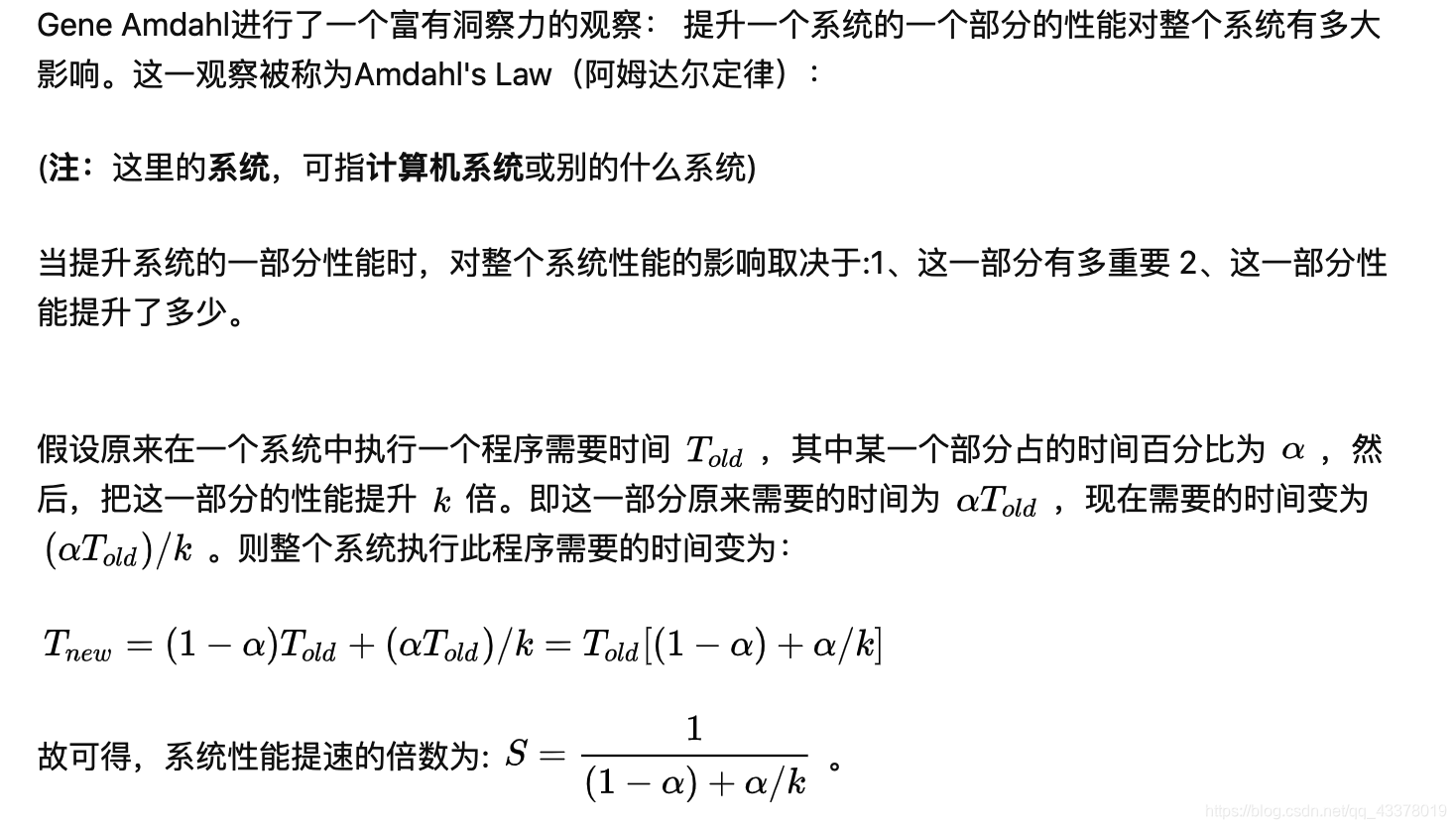
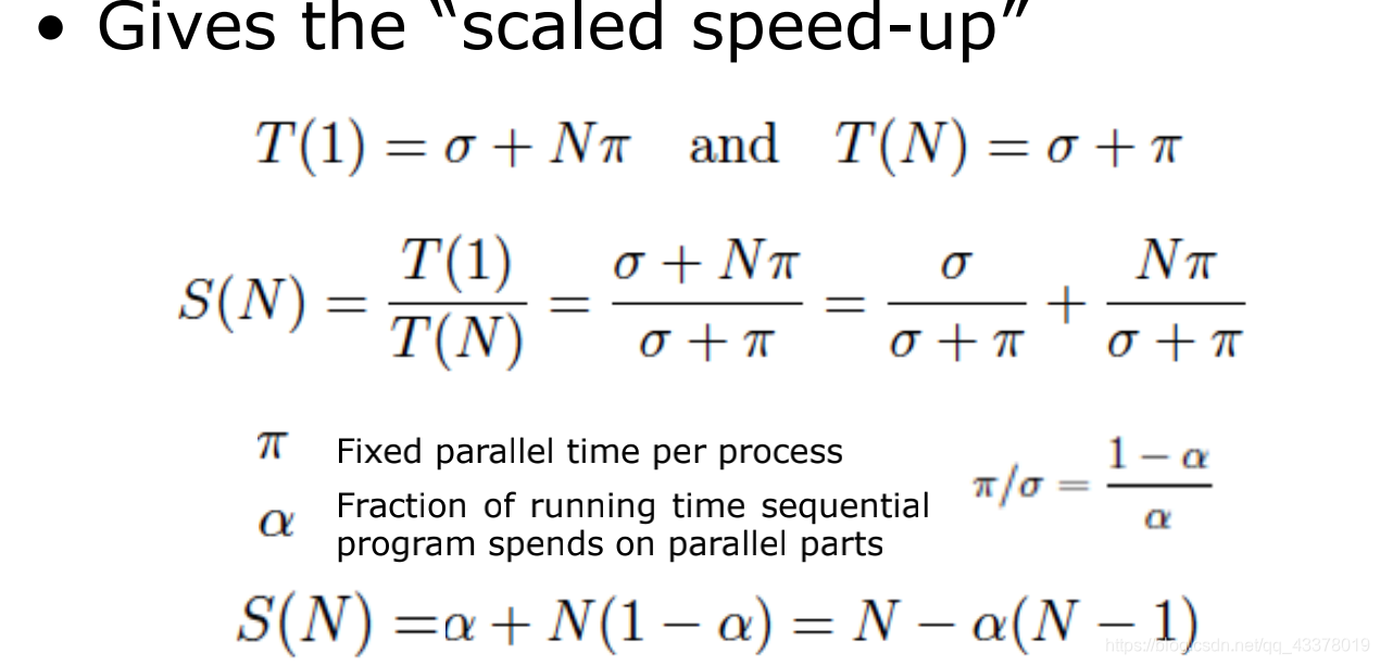
Gustafson-Barsis’s Law

阿姆达尔定用于计算算法并行化后可获得的最大预期改进：

Speedup = 1 / ( (1-p) + p/N )

其中 p 是代码的并行运行时间， N 是计算机核数；但此定律没有考虑到并行执行时的锁竞争、线程管理等消耗，最重要的是此定律没有考虑在计算机核数增加时，是否处理的数据也会更多，而只计算了固定核数固定任务的加速比。

古斯塔夫森定律相比于阿姆达尔定律，认为在计算机核数增加后所处理的任务就会更多，求解规模变大后串行代码运行时间是否会增加？

Speedup = p - a * ( p - 1 )

其中 p 是计算机核数， a 是串行代码执行时间所占百分比。

Speed up S using N processes is given as a linear formula dependent
on the number of processes and the fraction of time to run sequential
parts. Gustafson’s Law proposes that programmers tend to set the
size of problems to use the available equipment to solve problems
within a practical fixed time. Faster (more parallel) equipment
available, larger problems can be solved in the same time.