【OpenCV入门学习--python】直方图计算

例子源于OpenCV官网–直方图计算（https://docs.opencv.org/4.x/d8/dbc/tutorial_histogram_calculation.html）

使用OpenCV函数cv::split将图像分成相应的平面。
使用OpenCV函数cv::calcHist计算图像数组的直方图
使用函数cv::normalize对数组进行规范化

代码：

from __future__ import print_function
from __future__ import division
import cv2 as cv
import numpy as np
import argparse
#加载图像
parser = argparse.ArgumentParser(description='Code for Histogram Calculation tutorial.')
parser.add_argument('--input', help='Path to input image.', default='grass.jpg')
args = parser.parse_args()

src = cv.imread(cv.samples.findFile(args.input))
if src is None:
    print('Could not open or find the image:', args.input)
    exit(0)
#使用cv::split分离源图像在它的三个R,G和B平面:    
bgr_planes = cv.split(src)#我们的输入是要分割的图像(在这种情况下有三个通道)，输出是一个Mat向量


"""
现在我们准备开始为每个平面配置直方图。
由于我们处理的是B, G和R平面，我们知道我们的值将在区间[0,255]内
确定箱子的数量(5、10…):
"""

histSize = 256#设置值的范围(如我们所说，在0到255之间)

histRange = (0, 256) # 上边界是排他性的

accumulate = False#我们希望我们的箱子有相同的大小(统一)，并在一开始清除直方图，所以:

#使用cv::calcHist计算直方图:
b_hist = cv.calcHist(bgr_planes, [0], None, [histSize], histRange, accumulate=accumulate)
g_hist = cv.calcHist(bgr_planes, [1], None, [histSize], histRange, accumulate=accumulate)
r_hist = cv.calcHist(bgr_planes, [2], None, [histSize], histRange, accumulate=accumulate)

#创建一个图像来显示直方图:
hist_w = 512
hist_h = 400
bin_w = int(round( hist_w/histSize ))

histImage = np.zeros((hist_h, hist_w, 3), dtype=np.uint8)

#注意在绘图之前，首先对直方图进行规范化，使其值落在输入参数所指示的范围内:
cv.normalize(b_hist, b_hist, alpha=0, beta=hist_h, norm_type=cv.NORM_MINMAX)
cv.normalize(g_hist, g_hist, alpha=0, beta=hist_h, norm_type=cv.NORM_MINMAX)
cv.normalize(r_hist, r_hist, alpha=0, beta=hist_h, norm_type=cv.NORM_MINMAX)

#观察访问bin(在这种情况下，在这个1D-Histogram):#bin_w()是设置线的参数
for i in range(1, histSize):
    cv.line(histImage, ( bin_w*(i-1), hist_h - int(b_hist[i-1]) ),
            ( bin_w*(i), hist_h - int(b_hist[i]) ),
            ( 255, 0, 0), thickness=2)
    cv.line(histImage, ( bin_w*(i-1), hist_h - int(g_hist[i-1]) ),
            ( bin_w*(i), hist_h - int(g_hist[i]) ),
            ( 0, 255, 0), thickness=2)
    cv.line(histImage, ( bin_w*(i-1), hist_h - int(r_hist[i-1]) ),
            ( bin_w*(i), hist_h - int(r_hist[i]) ),
            ( 0, 0, 255), thickness=2)
    
    
cv.imshow('Source image', src)
cv.imshow('calcHist Demo', histImage)
cv.waitKey()

运行结果：

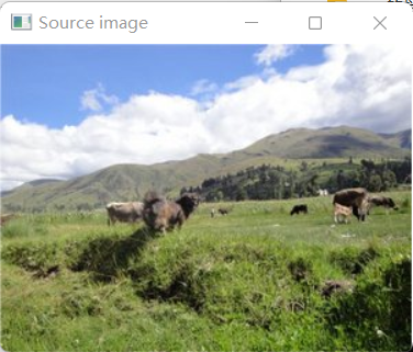
原图：

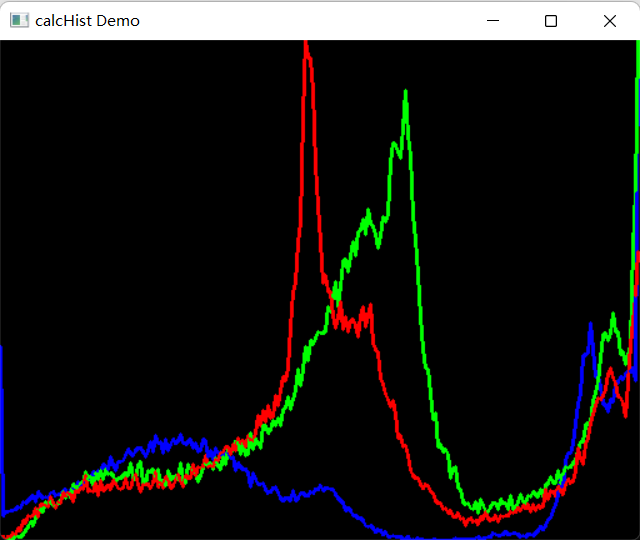
红绿蓝直方图：