


线性回归+基础优化算法
首先导入包
%matplotlib inline
import math
import time
import numpy as np
import torch
from d2l import torch as d2l
定义两个向量
n = 10000
a = torch.ones(n)
b = torch.ones(n)
定义一个计时器来比较循环和使用重载的+运算符计算的时长差别
class Timer:
    def __init__(self):
        self.times = []
        self.start()

    def start(self):
        self.tik = time.time()

    def stop(self):
        self.times.append(time.time() - self.tik())
        return self.times[:-1]

    def avg(self):
        return sum(self.times) / len(self.times)

    def sum(self):
        return sum(self.times)

    def cumsum(self):
        return np.array(self.times).cumsum().tolist
for循环
c = torch.zeros(n)
timer = Timer()
for i in range(n):
    c[i] = a[i] + b[i]
f'耗时 {timer.stop():.5f} sec'
重载+
timer.start()
d = a + b
f'耗时 {timer.stop():.5f} sec'
正态分布
def normal(x,mu,sigma):
     p = 1/math.sqrt(2*math.pi * sigma ** 2)
     return p * np.exp(-0.5/sigma ** 2 * (x - mu)**2)
可视化一个在(-10,10)上的正态分布
x = np.arange(-10,10,0.01)
params = [(0,1),(0,2),(3,1)]
d2l.plot(x,[normal(x,mu,sigma) for mu,sigma in params],xlabel='x',
         ylabel='p(x)',figsize=(4.5,2.5),
         legend = [f'mean {mu},std{sigma}' for mu,sigma in params])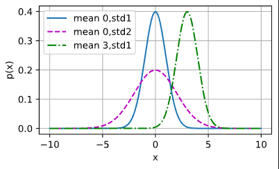
线性回归从零实现
构造一个人造数据集
def synthetic_data(w, b, num_examples):
    X = torch.normal(0, 1, (num_examples, len(w)))
    y = torch.matmul(X, w) + b
    y += torch.normal(0, 0.01, y.shape)
    return X, y.reshape((-1, 1))

true_w = torch.tensor([2, -3.4])
true_b = 4.2
features, labels = synthetic_data(true_w, true_b, 1000)
features 中的每一行都包含一个二维数据样本,labels 中的每一行都包含一维标签值
print('features:', features[0], '\nlabel:', labels[0])
可视化
d2l.set_figsize()
d2l.plt.scatter(features[:,(1)].detach().numpy(),labels.detach().numpy(),1)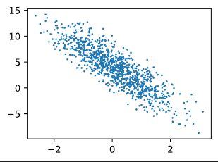
定义一个data_iter 函数
import random

def data_iter(batch_size,features,labels):
    num_examples = len(features)
    indices = list(range(num_examples))
    random.shuffle(indices)

    for i in range(0,num_examples,batch_size):
        batch_indices = torch.tensor(
            indices[i:min(i + batch_size,num_examples)]
        )
        yield features[batch_indices],labels[batch_indices]


batch_size = 10
for X,y in data_iter(batch_size,features,labels):
    print(X,'\n',y)
    break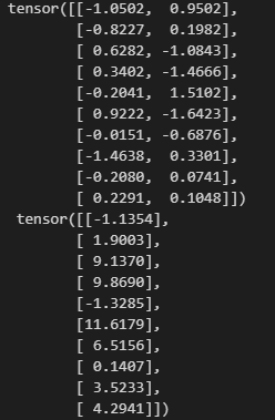
初始化模型参数
w = torch.normal(0,0.01,size=(2,1),requires_grad=True)
b = torch.zeros(1,requires_grad=True)
定义线性回归模型
def linreg(X,w,b):
    return torch.matmul(X,w) + b
定义均方损失函数
def squared_loss(y_hat,y):
    return(y_hat - y.reshape(y_hat.shape)) **2 / 2
定义sgd优化算法
def sgd(params , lr, batch_size):
    with torch.no_grad():
        for param in params:
            param -= lr * param.grad / batch_size
            param.grad.zero_()
训练
lr = 0.01
num_epochs = 5
net = linreg
loss = squared_loss

for epoch in range(num_epochs):
    for X,y in data_iter(batch_size, features, labels):
        l = loss(net(X,w,b),y)
        l.sum().backward()
        sgd([w,b],lr,batch_size)
    with torch.no_grad():
        train_l = loss(net(features,w,b),labels)
        print(f'epoch{epoch + 1},loss {float(train_l.mean()):f}')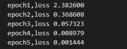
比较真实参数和通过训练学到的参数
print(f'w的估计误差:{true_w - w.reshape(true_w.shape)}')
print(f'b的估计误差:{true_b - b}')
线性回归的简洁实现
定义数据迭代器
from torch.utils import data
def load_array(data_arrays, batch_size,is_train = True):
    dataset = data.TensorDataset(*data_arrays)
    return data.DataLoader(dataset,batch_size,shuffle=is_train)
batch_size = 10
data_iter = load_array((features,labels),batch_size)
next(iter(data_iter))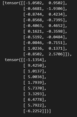
使用pytorch框架的预定义层并初始化参数
from torch import nn

net = nn.Sequential(nn.Linear(2,1))
net[0].weight.data.normal_(0,0.01)
net[0].bias.data.fill_(0)
初始化损失函数和SGD
loss = nn.MSELoss()
trainer = torch.optim.SGD(net.parameters(),lr = 0.03)
训练
num_epochs = 5
for epoch in range(num_epochs):
    for X,y in data_iter:
        l = loss(net(X),y)
        trainer.zero_grad()
        l.backward()
        trainer.step()

    l = loss(net(features),labels)
    print(f'epoch{epoch + 1}, loss{l:f}')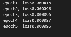
比较一下
w = net[0].weight.data
print('w的估计误差:', true_w - w.reshape(true_w.shape))
b = net[0].bias.data
print('b的估计误差:', true_b - b)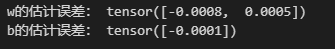
MNIST图像分类
定义数据集下载(由于之前已经有Fashion-MNIST数据集了,所以download= False)
trans = transforms.ToTensor ()
mnist_train = torchvision.datasets.FashionMNIST(
    root = "../data",train = True, download = False,transform = trans)
mnist_test = torchvision.datasets.FashionMNIST(
    root = "../data",train = False,download = False,transform = trans)
len(mnist_train),len(mnist_test)
mnist_train[0][0].shape
可视化数据集
def get_fashion_mnist_labels(labels):
    """返回Fashion-MNIST数据集的文本标签。"""
    text_labels = [
        't-shirt', 'trouser', 'pullover', 'dress', 'coat', 'sandal', 'shirt',
        'sneaker', 'bag', 'ankle boot']
    return [text_labels[int(i)] for i in labels]
def show_images(imgs, num_rows, num_cols, titles=None, scale=1.5):
"""Plot a list of images."""
figsize = (num_cols * scale, num_rows * scale)
_, axes = d2l.plt.subplots(num_rows, num_cols, figsize=figsize)
axes = axes.flatten()
for i, (ax, img) in enumerate(zip(axes, imgs)):
if torch.is_tensor(img):
ax.imshow(img.numpy())
else:
ax.imshow(img)
ax.axes.get_xaxis().set_visible(False)
ax.axes.get_yaxis().set_visible(False)
if titles:
ax.set_title(titles[i])
return axes看看样本图像及对应标签
X, y = next(iter(data.DataLoader(mnist_train, batch_size=28)))
show_images(X.reshape(28, 28, 28), 2, 14, titles=get_fashion_mnist_labels(y));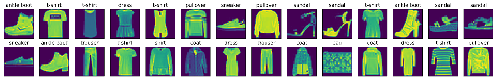
读取一批样本
batch_size = 256

def get_dataloader_workers():
    return 4

train_iter = data.DataLoader(mnist_train,batch_size,shuffle=True,num_workers=get_dataloader_workers())
timer = d2l.Timer()
for X, y in train_iter:
    continue
f'{timer.stop():.2f} sec'
softmax回归从零开始实现
展平图像 看作长度为784的向量 由于数据集有10个类别 故输出维度为10
from IPython import display

batch_size = 256
train_iter, test_iter = d2l.load_data_fashion_mnist(batch_size)
num_inputs = 784
num_outputs = 10

W = torch.normal(0, 0.01, size=(num_inputs, num_outputs), requires_grad=True)
b = torch.zeros(num_outputs, requires_grad=True)
定义softmax回归函数
def softmax(X):
    X_exp = torch.exp(X)
    partition = X_exp.sum(1,keepdim = True)
    return X_exp/partition
将每个元素变为非负数
X = torch.normal(0, 1, (2, 5))
X_prob = softmax(X)
X_prob, X_prob.sum(1)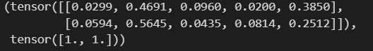
实现softmax回归模型
def net(X):
    return softmax(torch.matmul(X.reshape((-1,W.shape[0])),W) + b)
创建一个数据y_hat,其中包含2个样本在3个类别的预测概率, 使用y作为y_hat中概率的索引
y = torch.tensor([0, 2])
y_hat = torch.tensor([[0.1, 0.3, 0.6], [0.3, 0.2, 0.5]])
y_hat[[0, 1], y]
定义交叉熵损失函数
def cross_entropy(y_hat, y):
    return -torch.log(y_hat[range(len(y_hat)), y])

cross_entropy(y_hat, y)
将预测类别与真实 y 元素进行比较
def accuracy(y_hat, y):
    if len(y_hat.shape) > 1 and y_hat.shape[1] > 1:
        y_hat = y_hat.argmax(axis=1)
    cmp = y_hat.type(y.dtype) == y
    return float(cmp.type(y.dtype).sum())

accuracy(y_hat, y) / len(y)
评估在任意模型 net 的准确率
def evaluate_accuracy(net, data_iter):
    if isinstance(net, torch.nn.Module):
        net.eval()
    metric = Accumulator(2)
    for X, y in data_iter:
        metric.add(accuracy(net(X), y), y.numel())
    return metric[0] / metric[1]
Accumulator 实例中创建了 2 个变量,用于分别存储正确预测的数量和预测的总数量
class Accumulator:
    """在`n`个变量上累加。"""
    def __init__(self, n):
        self.data = [0.0] * n

    def add(self, *args):
        self.data = [a + float(b) for a, b in zip(self.data, args)]

    def reset(self):
        self.data = [0.0] * len(self.data)

    def __getitem__(self, idx):
        return self.data[idx]
Softmax回归的训练
def train_epoch_ch3(net, train_iter, loss, updater):
    """训练模型一个迭代周期(定义见第3章)。"""
    if isinstance(net, torch.nn.Module):
        net.train()
    metric = Accumulator(3)
    for X, y in train_iter:
        y_hat = net(X)
        l = loss(y_hat, y)
        if isinstance(updater, torch.optim.Optimizer):
            updater.zero_grad()
            l.backward()
            updater.step()
            metric.add(
                float(l) * len(y), accuracy(y_hat, y),
                y.size().numel())
        else:
            l.sum().backward()
            updater(X.shape[0])
            metric.add(float(l.sum()), accuracy(y_hat, y), y.numel())
    return metric[0] / metric[2], metric[1] / metric[2]
定义一个在动画中绘制数据的实用程序类
class Animator:
    """在动画中绘制数据。"""
    def __init__(self, xlabel=None, ylabel=None, legend=None, xlim=None,
                 ylim=None, xscale='linear', yscale='linear',
                 fmts=('-', 'm--', 'g-.', 'r:'), nrows=1, ncols=1,
                 figsize=(3.5, 2.5)):
        if legend is None:
            legend = []
        d2l.use_svg_display()
        self.fig, self.axes = d2l.plt.subplots(nrows, ncols, figsize=figsize)
        if nrows * ncols == 1:
            self.axes = [self.axes,]
        self.config_axes = lambda: d2l.set_axes(self.axes[
            0], xlabel, ylabel, xlim, ylim, xscale, yscale, legend)
        self.X, self.Y, self.fmts = None, None, fmts

    def add(self, x, y):
        if not hasattr(y, "__len__"):
            y = [y]
        n = len(y)
        if not hasattr(x, "__len__"):
            x = [x] * n
        if not self.X:
            self.X = [[] for _ in range(n)]
        if not self.Y:
            self.Y = [[] for _ in range(n)]
        for i, (a, b) in enumerate(zip(x, y)):
            if a is not None and b is not None:
                self.X[i].append(a)
                self.Y[i].append(b)
        self.axes[0].cla()
        for x, y, fmt in zip(self.X, self.Y, self.fmts):
            self.axes[0].plot(x, y, fmt)
        self.config_axes()
        display.display(self.fig)
        display.clear_output(wait=True)
训练函数
def train_ch3(net, train_iter, test_iter, loss, num_epochs, updater):
    """训练模型(定义见第3章)。"""
    animator = Animator(xlabel='epoch', xlim=[1, num_epochs], ylim=[0.3, 0.9],
                        legend=['train loss', 'train acc', 'test acc'])
    for epoch in range(num_epochs):
        train_metrics = train_epoch_ch3(net, train_iter, loss, updater)
        test_acc = evaluate_accuracy(net, test_iter)
        animator.add(epoch + 1, train_metrics + (test_acc,))
    train_loss, train_acc = train_metrics
    assert train_loss < 0.5, train_loss
    assert train_acc <= 1 and train_acc > 0.7, train_acc
    assert test_acc <= 1 and test_acc > 0.7, test_acc
小批量随机梯度下降来优化模型的损失函数
lr = 0.1

def updater(batch_size):
    return d2l.sgd([W, b], lr, batch_size)
训练模型10个迭代周期
num_epochs = 10
train_ch3(net, train_iter, test_iter, cross_entropy, num_epochs, updater)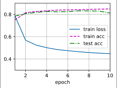
对图像进行分类预测
def predict_ch3(net, test_iter, n=10):
    """预测标签(定义见第3章)。"""
    for X, y in test_iter:
        break
    trues = d2l.get_fashion_mnist_labels(y)
    preds = d2l.get_fashion_mnist_labels(net(X).argmax(axis=1))
    titles = [true + '\n' + pred for true, pred in zip(trues, preds)]
    d2l.show_images(X[0:n].reshape((n, 28, 28)), 1, n, titles=titles[0:n])

predict_ch3(net, test_iter)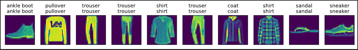
softmax回归的简洁实现
Softmax 回归的输出层是一个全连接层
batch_size = 256
train_iter, test_iter = d2l.load_data_fashion_mnist(batch_size)
net = nn.Sequential(nn.Flatten(), nn.Linear(784, 10))

def init_weights(m):
    if type(m) == nn.Linear:
        nn.init.normal_(m.weight, std=0.01)

net.apply(init_weights);
在交叉熵损失函数中传递未归一化的预测,并同时计算softmax及其对数
loss = nn.CrossEntropyLoss()使用学习率为0.1的小批量随机梯度下降作为优化算法
trainer = torch.optim.SGD(net.parameters(), lr=0.1)调用之前定义的训练函数来训练模型
num_epochs = 15
d2l.train_ch3(net, train_iter, test_iter, loss, num_epochs, trainer)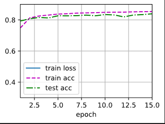


 10万+
10万+

 被折叠的 条评论
为什么被折叠?
被折叠的 条评论
为什么被折叠?
 到【灌水乐园】发言


