MIND——Modality independent neighbourhood descriptor 模态无关邻域描述符

参考：

https://blog.mbedded.ninja/programming/signal-processing/image-processing/image-registration/modality-independent-neighbourhood-descriptor-mind/

《MIND: Modality independent neighbourhood descriptor for multi-modal deformable registration》论文

2D版的MIND_shchojj的博客-CSDN博客

MIND（模态独立邻域描述符）是一种图像配准算法，旨在提取每个像素/体素周围局部区域的结构信息。

一、原理介绍

1、公式介绍

MIND表达式如下：

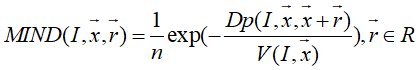
Dp(I,x,x+r)指以x点为中心的Patch块和以x+r为中心的Patch块的距离，即两个Patch块之差的平方。

V(I,x)是指图像中x点的6邻域搜索空间内各点的Dp(I,x,x+r)相加再平均。(这个邻域搜索空间后面介绍)

MIND(I,x,r)是感兴趣点x的邻域搜索空间内这n个点的Dp(I,x,x+r)除以该点的V(I,x)，再负对数。

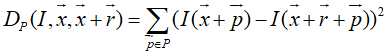
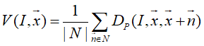
邻域搜索空间neigh Search Space:分为三种

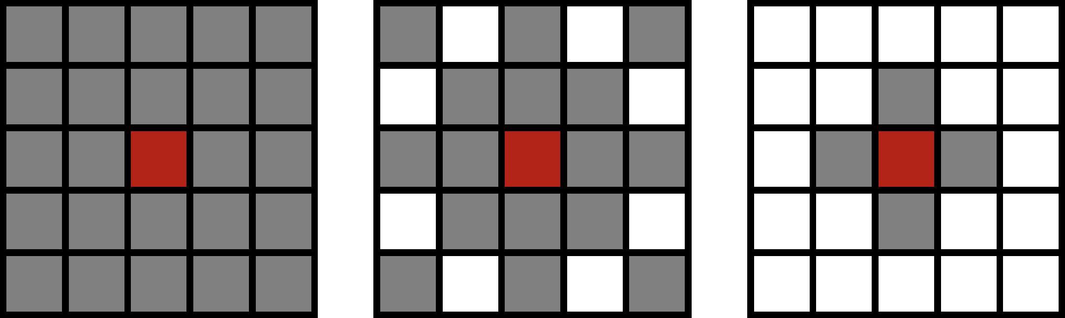
紧密型采样（全采样） 稀疏性采样（45°采样） 6邻域采样

*红色小块为感兴趣点，即需要求MIND特征的像素点。

如果设置一个5*5的一个neigh,紧密型采样的邻域搜索空间包括除红色像素以外的所有灰色像素点；稀疏型采样同理如中图所示；6邻域采样应该是文章针对三维图像来讲的，对于二维的图像，应该也可以说是4邻域。

Patch:3*3的patch是指一个3*3的像素小块

2、图示说明

从一个5*5的像素块开始理解：

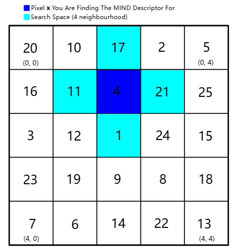
*蓝色像素4的地方是感兴趣点，即正要计算MIND特征的像素点，

*靛青色像素是设置的4邻域搜索空间

开始计算之前，先设置参数patch(3*3),neigh(3*3,4邻域采样)

（1）4邻域搜索空间内各点的Dp(I,x,x+r)

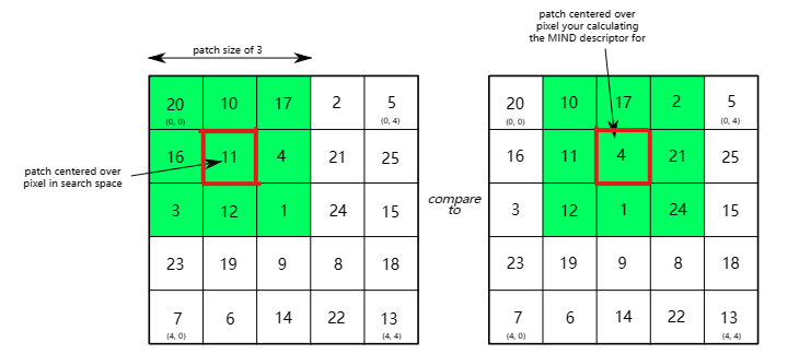
向量x=(1,2)，向量x+r={(1,1),(0,2),(1,3),(2,2)}

同理求完四个点的Dp(I,x,x+r)如下图所示：

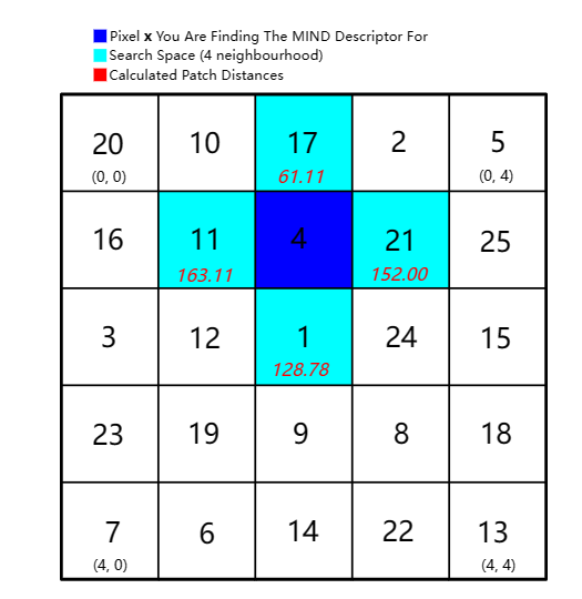
（2）求V(I,x)

V(I,x)在2维图像中需要求4邻域搜索空间的4个点的Dp(I,x,x+r)的平均

到这里只求得了一个像素点（1,2）的V(I,x)，对于整个5*5的像素块或者256*256的图像，我们就需要求出这个像素块或者图像的V(I,x)的一个矩阵。

array([[ 15.33,  41.97,  68.19,  87.61,  60.97],
       [ 47.06,  93.78, 126.25, 137.28,  90.56],
       [ 93.72, 141.75, 157.06, 129.78,  81.75],
       [109.42, 147.36, 152.08,  99.03,  61.08],
       [ 77.69,  95.56,  94.03,  49.36,  31.5 ]])

（3）计算MIND特征

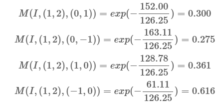
那么MIND(I,(1,2))=[0.300,0.275,0.361,0.616]

同样到这里，我们只获得了点（1，2）的MIND特征，而对于这个5*5的像素块，我们还要获得其余24个点的MIND特征。

最终得到的这个5*5的像素块的MIND特征如下：

mind_descriptors =
  array([
       [[0.199, 0.404, 0.258, 0.884],
        [0.142, 0.554, 0.381, 0.611],
        [0.354, 0.301, 0.408, 0.421],
        [0.505, 0.446, 0.265, 0.307],
        [0.955, 0.374, 0.205, 0.25 ]],

       [[0.367, 0.615, 0.126, 0.643],
        [0.176, 0.604, 0.266, 0.649],
        [0.3  , 0.275, 0.361, 0.616],
        [0.395, 0.33 , 0.328, 0.428],
        [0.878, 0.244, 0.248, 0.344]],

       [[0.43 , 0.845, 0.142, 0.354],
        [0.301, 0.572, 0.255, 0.416],
        [0.326, 0.339, 0.377, 0.44 ],
        [0.419, 0.257, 0.552, 0.308],
        [0.765, 0.251, 0.445, 0.214]],

       [[0.49 , 0.887, 0.224, 0.188],
        [0.376, 0.589, 0.308, 0.269],
        [0.349, 0.388, 0.371, 0.365],
        [0.383, 0.199, 0.525, 0.46 ],
        [0.621, 0.211, 0.413, 0.339]],

       [[0.488, 0.948, 0.325, 0.121],
        [0.518, 0.558, 0.39 , 0.162],
        [0.432, 0.512, 0.412, 0.201],
        [0.575, 0.202, 0.575, 0.274],
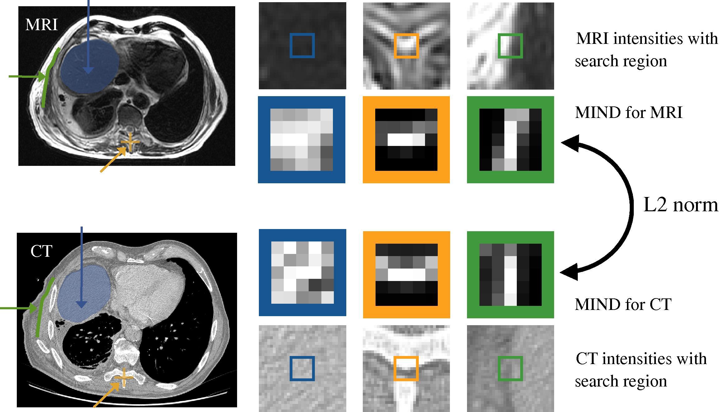
        [0.528, 0.42 , 0.459, 0.18 ]]])

如果想要比较一个5*5和像素块A和一个5*5的像素块B的结构相似性，那么就要先获得A和B的形状为（5,5,4）的MIND特征矩阵。然后将每个像素点的对应的MIND矩阵加和作为该像素点的MIND特征，最后就又会得到A的5*5的MIND特征图和B的MIND特征图。论文中的MIND特征图展示如下：

二、Python实现代码Pytorch（2D版）

import torch
import numpy as np
import torchvision
import SimpleITK as sitk
import torch.nn.functional as F
import matplotlib.pyplot as plt
def gaussian_kernel(sigma, sz):
    xpos_vec = np.arange(sz)
    ypos_vec = np.arange(sz)
    output = np.ones([1, 1,sz, sz], dtype=np.single)
    midpos = sz // 2
    for xpos in xpos_vec:
        for ypos in ypos_vec:
            output[:,:,xpos,ypos] = np.exp(-((xpos-midpos)**2 + (ypos-midpos)**2) / (2 * sigma**2)) / (2 * np.pi * sigma**2)
    return output
def torch_image_translate(input_, tx, ty, interpolation='nearest'):
    # got these parameters from solving the equations for pixel translations
    # on https://www.tensorflow.org/api_docs/python/tf/contrib/image/transform
    translation_matrix = torch.zeros([1, 3, 3], dtype=torch.float)
    translation_matrix[:, 0, 0] = 1.0
    translation_matrix[:, 1, 1] = 1.0
    translation_matrix[:, 0, 2] = -2*tx/(input_.size()[2]-1)
    translation_matrix[:, 1, 2] = -2*ty/(input_.size()[3]-1)
    translation_matrix[:, 2, 2] = 1.0
    grid = F.affine_grid(translation_matrix[:, 0:2, :], input_.size()).to(input_.device)
    wrp = F.grid_sample(input_, grid, mode=interpolation)
    return wrp
def Dp(image, xshift, yshift, sigma, patch_size):
    shift_image = torch_image_translate(image, xshift, yshift, interpolation='nearest')#将image在x、y方向移动I`(a)
    diff = torch.sub(image, shift_image)#计算差分图I-I`(a)
    diff_square = torch.mul(diff, diff)#(I-I`(a))^2
    res = torch.conv2d(diff_square, weight =torch.from_numpy(gaussian_kernel(sigma, patch_size)), stride=1, padding=3)#C*(I-I`(a))^2
    return res
 
def MIND(image, patch_size, neigh_size, sigma, eps,image_size0,image_size1,  name='MIND'):
    # compute the Modality independent neighbourhood descriptor (MIND) of input image.
    # suppose the neighbor size is R, patch size is P.
    # input image is 384 x 256 x input_c_dim
    # output MIND is (384-P-R+2) x (256-P-R+2) x R*R
    reduce_size = int((patch_size + neigh_size - 2) / 2)#卷积后减少的size
 
    # estimate the local variance of each pixel within the input image.
    Vimg = torch.add(Dp(image, -1, 0, sigma, patch_size), Dp(image, 1, 0, sigma, patch_size))
    Vimg = torch.add(Vimg, Dp(image, 0, -1, sigma, patch_size))
    Vimg = torch.add(Vimg, Dp(image, 0, 1, sigma, patch_size))#sum(Dp)
    Vimg = torch.div(Vimg,4) + torch.mul(torch.ones_like(Vimg), eps)#防除零
    # estimate the (R*R)-length MIND feature by shifting the input image by R*R times.
    xshift_vec = np.arange( -(neigh_size//2), neigh_size - (neigh_size//2))#邻域计算
    yshift_vec = np.arange(-(neigh_size // 2), neigh_size - (neigh_size // 2))#邻域计算
    iter_pos = 0
    for xshift in xshift_vec:
        for yshift in yshift_vec:
            if (xshift,yshift) == (0,0):
                continue
            MIND_tmp = torch.exp(torch.mul(torch.div(Dp(image, xshift, yshift,  sigma, patch_size), Vimg), -1))#exp(-D(I)/V(I))
            tmp = MIND_tmp[:, :, reduce_size:(image_size0 - reduce_size), reduce_size:(image_size1 - reduce_size)]
            if iter_pos == 0:
                output = tmp
            else:
                output = torch.cat([output,tmp], 1)
            iter_pos = iter_pos + 1
 
    # normalization.
    input_max, input_indexes = torch.max(output, dim=1)
    output = torch.div(output,input_max)
 
    return output
def abs_criterion(in_, target):
    return torch.mean(torch.abs(in_ - target))
if __name__ == '__main__':
    patch_size=7
    neigh_size=9
    sigma=2.0
    eps=1e-5
    image_size0=512
    image_size1=512
    ct_path = r'F:\dataset\coarseReg\00001_SRO1_ct_axial_drr.nii.gz'
    mr_path = r'F:\dataset\coarseReg\00001_SRO1_mr_axial_drr.nii.gz'
    ct_sitk = sitk.ReadImage(ct_path,sitk.sitkFloat32)
    mr_sitk = sitk.ReadImage(mr_path,sitk.sitkFloat32)
 
    ct_axial_drr = sitk.GetArrayFromImage(ct_sitk)[np.newaxis ,np.newaxis,:,:]
    mr_axial_drr = sitk.GetArrayFromImage(mr_sitk)[np.newaxis ,np.newaxis,:,: ]
 
    plt.imshow(ct_axial_drr.squeeze())
    plt.show()
 
    ct_axial_drr = torch.from_numpy(ct_axial_drr)
    mr_axial_drr = torch.from_numpy(mr_axial_drr)
 
    A_MIND = MIND(ct_axial_drr,  patch_size, neigh_size, sigma, eps,image_size0,image_size1,  name='realA_MIND')
    B_MIND = MIND(mr_axial_drr,  patch_size, neigh_size, sigma, eps,image_size0,image_size1,  name='realA_MIND')
    g_loss_MIND = abs_criterion(A_MIND, B_MIND)
    print('g_loss_MIND', g_loss_MIND)
 
    # tf =  np.load( r"C:\Users\shcho\Desktop\validation\tf.npy" )
    # tc =  np.load( r"C:\Users\shcho\Desktop\validation\tc.npy" )
 
    # plt.imshow(tf)
    # plt.show()
    # plt.imshow(tc)
    # plt.show()
    # print(tf.shape, tc.shape)
    #
    # # print(tf.transpose((2,0,1)).shape, tc.shape)
    # t = tf.transpose((2,0,1)) -tc
    #
    # # t = tf -tc
    #
    # print(np.max(t))

可以通过上面代码提取整张图像的MIND特征，且该函数可以被用于基于CycleGAN网络处理MRtoCT图像的损失函数并得到很好的结果，如论文《Unsupervised MR-to-CT Synthesis using Structure Constrained CycleGAN》所述，同理可用于相似的CycleGAN网络模型处理医学图像的任务中来约束A，B域的结构信息。