SINetv2：Concealed Object Detection——论文简述

一、简介

目标检测可以分为三个类别：通用目标检测（语义分割、全景分割）、突出目标检测和伪装目标检测。

与上一篇文章一样，同样是伪装目标检测，但是取得了更好的效果。

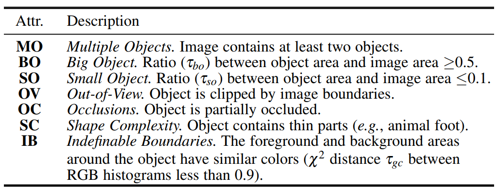
数据集采用COD10k，每张图片采用六种标注：属性（如下表所示）、类别（super-&sub-class）、bounding boxes、object
annotation、instance annotation 和 edge annotation。

较v1增加了neighbor connection decoder(NCD) 和 group-reversal attention (GRA)。

本论文完成的是目标层面的检测，而不是实例分割。

二、模型

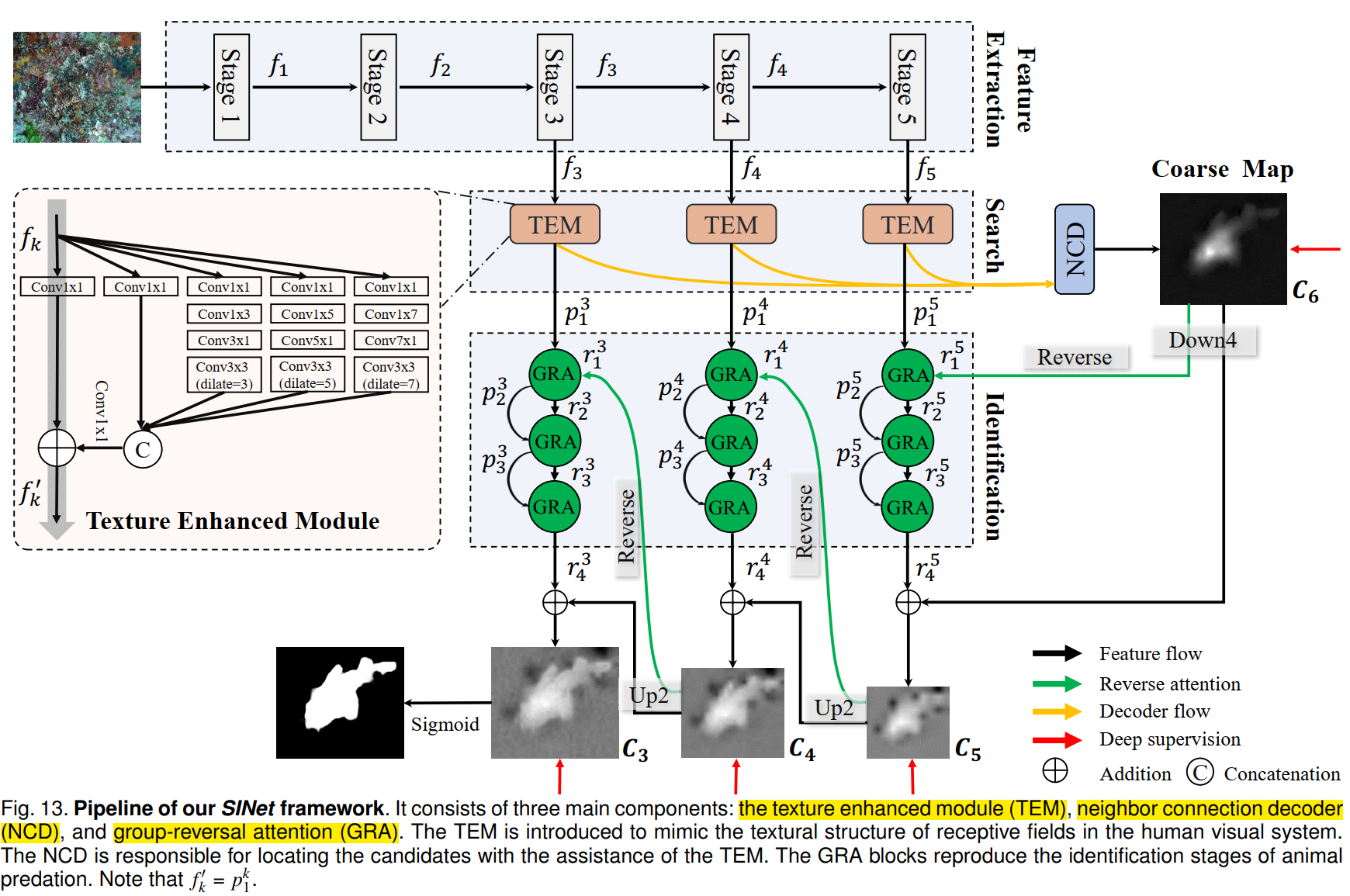
模型分为两个部分：搜索和确认。

2.1 搜索阶段

2.1.1 特征抽取

backbone是res2net50。

2.1.2 Texture Enhanced Module (TEM)

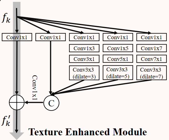
对应代码中的 Receptive Field Block，其中标准的 (2i - 1) x (2i - 1) 大小的卷积操作可以分为 1 x (2i - 1) 和 (2i - 1) x 1 大小的两个连续卷积操作，从而在不减小表征能力的前提下提高推理速度。

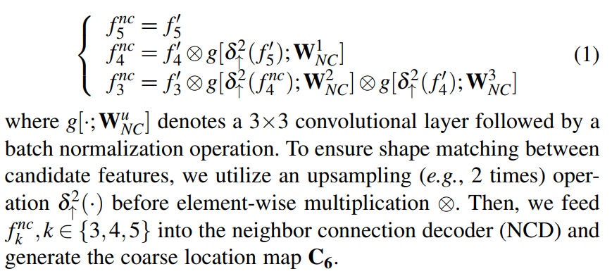
2.1.3 Neighbor Connection Decoder (NCD)

低层级的特征由于更大的空间分辨率，会消耗更多的计算资源，但是表现不佳，本论文采用最后三层特征，而不是将所有特征金字塔送入 NCD 中。

NCD 解决的问题是如何保持同一层内语义的一致性，以及如何在各层之间架起上下文的桥梁。

对送入 NCD 的三层特征再做一次处理，对应如下代码中的 xi_1(i = 1, 2, 3)，然后再是 NCD 操作。

    def forward(self, x1, x2, x3):
        x1_1 = x1  # f5
        x2_1 = self.conv_upsample1(self.upsample(x1)) * x2  # f4
        x3_1 = self.conv_upsample2(self.upsample(x2_1)) * self.conv_upsample3(self.upsample(x2)) * x3  # f3

        x2_2 = torch.cat((x2_1, self.conv_upsample4(self.upsample(x1_1))), 1)
        x2_2 = self.conv_concat2(x2_2)

        x3_2 = torch.cat((x3_1, self.conv_upsample5(self.upsample(x2_2))), 1)
        x3_2 = self.conv_concat3(x3_2)

        x = self.conv4(x3_2)
        x = self.conv5(x)

        return x

2.2 确认阶段

如下代码注释所示，标注了该模型示意图的确认阶段的节点。

# Neighbourhood Connected Decoder
        S_g = self.NCD(x4_rfb, x3_rfb, x2_rfb)  # C6
        S_g_pred = F.interpolate(S_g, scale_factor=8, mode='bilinear')    # Sup-1 (bs, 1, 44, 44) -> (bs, 1, 352, 352)

        # ---- reverse stage 5 ----
        guidance_g = F.interpolate(S_g, scale_factor=0.25, mode='bilinear')  # r1,5
        ra4_feat = self.RS5(x4_rfb, guidance_g)  # r4,5
        S_5 = ra4_feat + guidance_g   # C5
        S_5_pred = F.interpolate(S_5, scale_factor=32, mode='bilinear')  # Sup-2 (bs, 1, 11, 11) -> (bs, 1, 352, 352)

        # ---- reverse stage 4 ----
        guidance_5 = F.interpolate(S_5, scale_factor=2, mode='bilinear')  # r1,4
        ra3_feat = self.RS4(x3_rfb, guidance_5)  # r4,4
        S_4 = ra3_feat + guidance_5  # C4
        S_4_pred = F.interpolate(S_4, scale_factor=16, mode='bilinear')  # Sup-3 (bs, 1, 22, 22) -> (bs, 1, 352, 352)

        # ---- reverse stage 3 ----
        guidance_4 = F.interpolate(S_4, scale_factor=2, mode='bilinear')  # r1,3
        ra2_feat = self.RS3(x2_rfb, guidance_4)  # r4,3
        S_3 = ra2_feat + guidance_4  # C3
        S_3_pred = F.interpolate(S_3, scale_factor=8, mode='bilinear')   # Sup-4 (bs, 1, 44, 44) -> (bs, 1, 352, 352)

2.2.1 Reverse Guidance

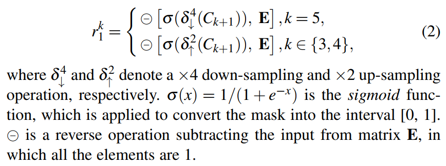
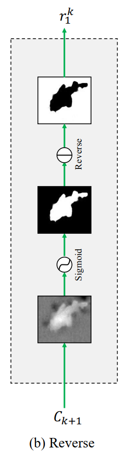
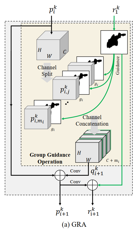
2.2.2 Group-Reversal Attention (GRA)

就是两个 chunk 和 cat 操作。