【MATLAB基础绘图第3棒】绘制散点密度图

1 方法一：scatplot函数

1.1 MATLAB函数

scatplot-Scatter plot with color indicating data density.
函数代码如下：

function out = scatplot(x,y,method,radius,N,n,po,ms)
% Scatter plot with color indicating data density
%
% USAGE:
%   out = scatplot(x,y,method,radius,N,n,po,ms)
%   out = scatplot(x,y,dd)
%
% DESCRIPTION:
%   Draws a scatter plot with a colorscale 
%   representing the data density computed 
%   using three methods
%
% INPUT VARIABLES:
%   x,y - are the data points
%   method - is the method used to calculate data densities:
%       'circles' - uses circles with a determined area 
%               centered at each data point
%       'squares' - uses squares with a determined area 
%               centered at each data point
%       'voronoi' - uses voronoi cells to determin data densities
%               default method is 'voronoi'
%   radius - is the radius used for the circles or squares
%       used to calculate the data densities if
%       (Note: only used in methods 'circles' and 'squares'
%           default radius is sqrt((range(x)/30)^2 + (range(y)/30)^2)
%   N - is the size of the square mesh (N x N) used to  
%       filter and calculate contours
%       default is 100
%   n - is the number of coeficients used in the 2-D
%       running mean filter
%       default is 5
%       (Note: if n is length(2), n(2) is tjhe number of
%       of times the filter is applied)
%   po - plot options:
%       0 - No plot
%       1 - plots only colored data points (filtered)
%       2 - plots colored data points and contours (filtered)
%       3 - plots only colored data points (unfiltered)
%       4 - plots colored data points and contours (unfiltered)
%           default is 1
%   ms - uses this marker size for filled circles
%       default is 4
%
% OUTPUT VARIABLE:
%   out - structure array that contains the following fields:
%       dd - unfiltered data densities at (x,y)
%       ddf - filtered data densities at (x,y)
%       radius - area used in 'circles' and 'squares'
%               methods to calculate densities
%       xi - x coordenates for zi matrix 
%       yi - y coordenates for zi matrix
%       zi - unfiltered data densities at (xi,yi)
%       zif - filtered data densities at (xi,yi)
%       [c,h] = contour matrix C as described in
%           CONTOURC and a handle H to a contourgroup object
%       hs = scatter points handles
%
%Copy-Left, Alejandro Sanchez-Barba, 2005

if nargin==0
    scatplotdemo
    return
end
if nargin<3 | isempty(method)
    method = 'vo';
end
if isnumeric(method)
   gsp(x,y,method,2)
   return
else
    method = method(1:2);
end
if nargin<4 | isempty(n)
    n = 5; %number of filter coefficients
end
if nargin<5 | isempty(radius)
    radius = sqrt((range(x)/30)^2 + (range(y)/30)^2);
end
if nargin<6 | isempty(po)
    po = 1; %plot option
end
if nargin<7 | isempty(ms)
    ms = 4; %markersize
end
if nargin<8 | isempty(N)
    N = 100; %length of grid
end
%Correct data if necessary
x = x(:);
y = y(:);
%Asuming x and y match
idat = isfinite(x);
x = x(idat);
y = y(idat);
holdstate = ishold;
if holdstate==0
    cla
end
hold on
%--------- Caclulate data density ---------
dd = datadensity(x,y,method,radius);
%------------- Gridding -------------------
xi = repmat(linspace(min(x),max(x),N),N,1);
yi = repmat(linspace(min(y),max(y),N)',1,N);
zi = griddata(x,y,dd,xi,yi);
%----- Bidimensional running mean filter -----
zi(isnan(zi)) = 0;
coef = ones(n(1),1)/n(1);
zif = conv2(coef,coef,zi,'same');
if length(n)>1
    for k=1:n(2)
        zif = conv2(coef,coef,zif,'same');
    end
end
%-------- New Filtered data densities --------
ddf = griddata(xi,yi,zif,x,y);
%----------- Plotting --------------------
switch po
    case {1,2}
        if po==2
            [c,h] = contour(xi,yi,zif);
            out.c = c;
            out.h = h;
        end %if
        hs = gsp(x,y,ddf,ms);
        out.hs = hs;
        colorbar
    case {3,4}
        if po>3
            [c,h] = contour(xi,yi,zi);
            out.c = c;
        end %if
        hs = gsp(x,y,dd,ms);
        out.hs = hs;
        colorbar    
end %switch
%------Relocate variables and place NaN's ----------
dd(idat) = dd;
dd(~idat) = NaN;
ddf(idat) = ddf;
ddf(~idat) = NaN;
%--------- Collect variables ----------------
out.dd = dd;
out.ddf = ddf;
out.radius = radius;
out.xi = xi;
out.yi = yi;
out.zi = zi;
out.zif = zif;
if ~holdstate
    hold off
end
return
%~~~~~~~~~~~~~~~~~~~~~~~~~~~~~~~~~~~~~~
function scatplotdemo
po = 2;
method = 'squares';
radius = [];
N = [];
n = [];
ms = 5;
x = randn(1000,1);
y = randn(1000,1);

out = scatplot(x,y,method,radius,N,n,po,ms);

return
%~~~~~~~~~~ Data Density ~~~~~~~~~~~~~~
function dd = datadensity(x,y,method,r)
%Computes the data density (points/area) of scattered points
%Striped Down version
%
% USAGE:
%   dd = datadensity(x,y,method,radius)
%
% INPUT:
%   (x,y) -  coordinates of points
%   method - either 'squares','circles', or 'voronoi'
%       default = 'voronoi'
%   radius - Equal to the circle radius or half the square width
Ld = length(x);
dd = zeros(Ld,1);
switch method %Calculate Data Density
    case 'sq'  %---- Using squares ----
        for k=1:Ld
            dd(k) = sum( x>(x(k)-r) & x<(x(k)+r) & y>(y(k)-r) & y<(y(k)+r) );
        end %for
        area = (2*r)^2;
        dd = dd/area;
    case 'ci'
        for k=1:Ld
            dd(k) = sum( sqrt((x-x(k)).^2 + (y-y(k)).^2) < r );
        end
        area = pi*r^2;
        dd = dd/area;
    case 'vo'  %----- Using voronoi cells ------
        [v,c] = voronoin([x,y]);     
        for k=1:length(c) 
            %If at least one of the indices is 1, 
            %then it is an open region, its area
            %is infinity and the data density is 0
            if all(c{k}>1)   
                a = polyarea(v(c{k},1),v(c{k},2));
                dd(k) = 1/a;
            end %if
        end %for
end %switch
return
%~~~~~~~~~~ Graf Scatter Plot ~~~~~~~~~~~
function varargout = gsp(x,y,c,ms)
%Graphs scattered poits
map = colormap;
ind = fix((c-min(c))/(max(c)-min(c))*(size(map,1)-1))+1;
h = [];
%much more efficient than matlab's scatter plot
for k=1:size(map,1) 
    if any(ind==k)
        h(end+1) = line('Xdata',x(ind==k),'Ydata',y(ind==k), ...
            'LineStyle','none','Color',map(k,:), ...
            'Marker','.','MarkerSize',ms);
    end
end
if nargout==1
    varargout{1} = h; 
end
return

语法：

1.2 案例

MATLAB代码如下：

clc
close all
clear
%% 导入数据
X=[
    -0.752713846442762  2.48140797998545    1
...
-1.62181912776895   -0.851506362212275  2
];

%% 绘图
figure(1)
box on;
scatplot(X(:,1),X(:,2),'circles', sqrt((range(X(:, 1))/30)^2 + (range(X(:,2))/30)^2), 100, 5, 1, 8);
xlabel("X");
ylabel("Y");
% colormap jet
print(gcf,'-dpng','散点密度图.png');

图形如下：

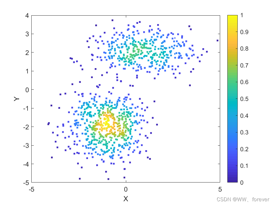
若调用函数参数为空，则得到以下图形：

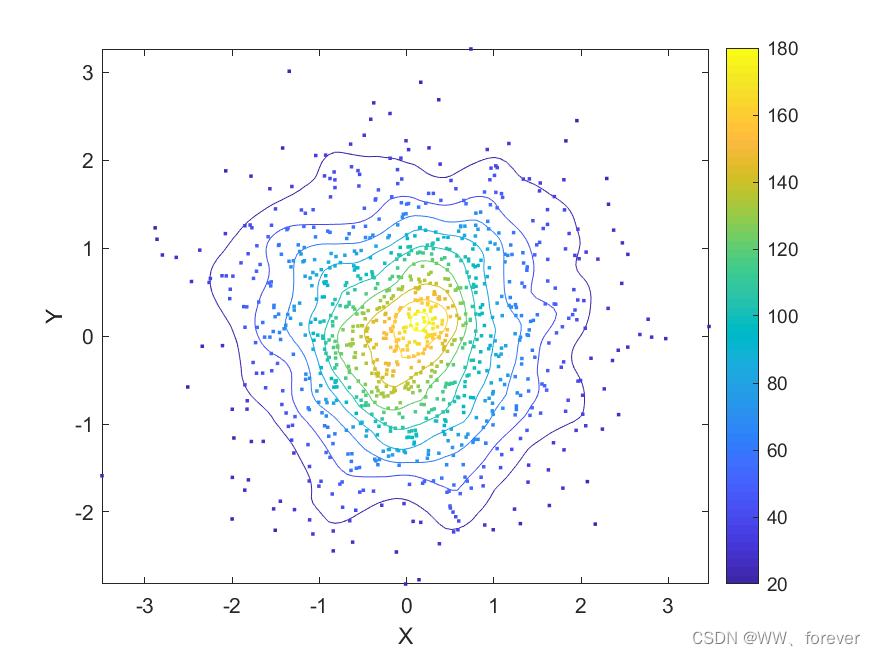
另：可对函数代码进行修正，不显示colormap

2 方法二：

2.1 案例

MATLAB代码如下：

clc
close all
clear
%% 导入数据
X=[
    -0.752713846442762  2.48140797998545    1
...
-1.62181912776895   -0.851506362212275  2
];
%%
datamin = min(min(XYZ(:, 1)), min(XYZ(:, 2)));
datamax = max(max(XYZ(:, 1)), max(XYZ(:, 2)));
datamin = floor(datamin);
datamax = ceil(datamax);

Length = 600;
Width = 600;

axismin = datamin;
axismax = datamax;

% 绘制密度图
XYZ(:, 3) = XYZ(:, 3) - XYZ(:, 3);
sizeXYZ = size(XYZ);
searchR = 1.0;
for i = 1 : sizeXYZ(1)
    index_i = find(XYZ(:, 1) > XYZ(i, 1) - searchR & XYZ(:, 1) < XYZ(i, 1) + searchR ...
        & XYZ(:, 2) > XYZ(i, 2) - searchR & XYZ(:, 2) < XYZ(i, 2) + searchR);
    sizeIndexI = size(index_i);
    XYZ(i, 3) = sizeIndexI(1);
end
[sortXYZ, sortI] = sort(XYZ(:, 3));

figure(1)
hold on;
box on;
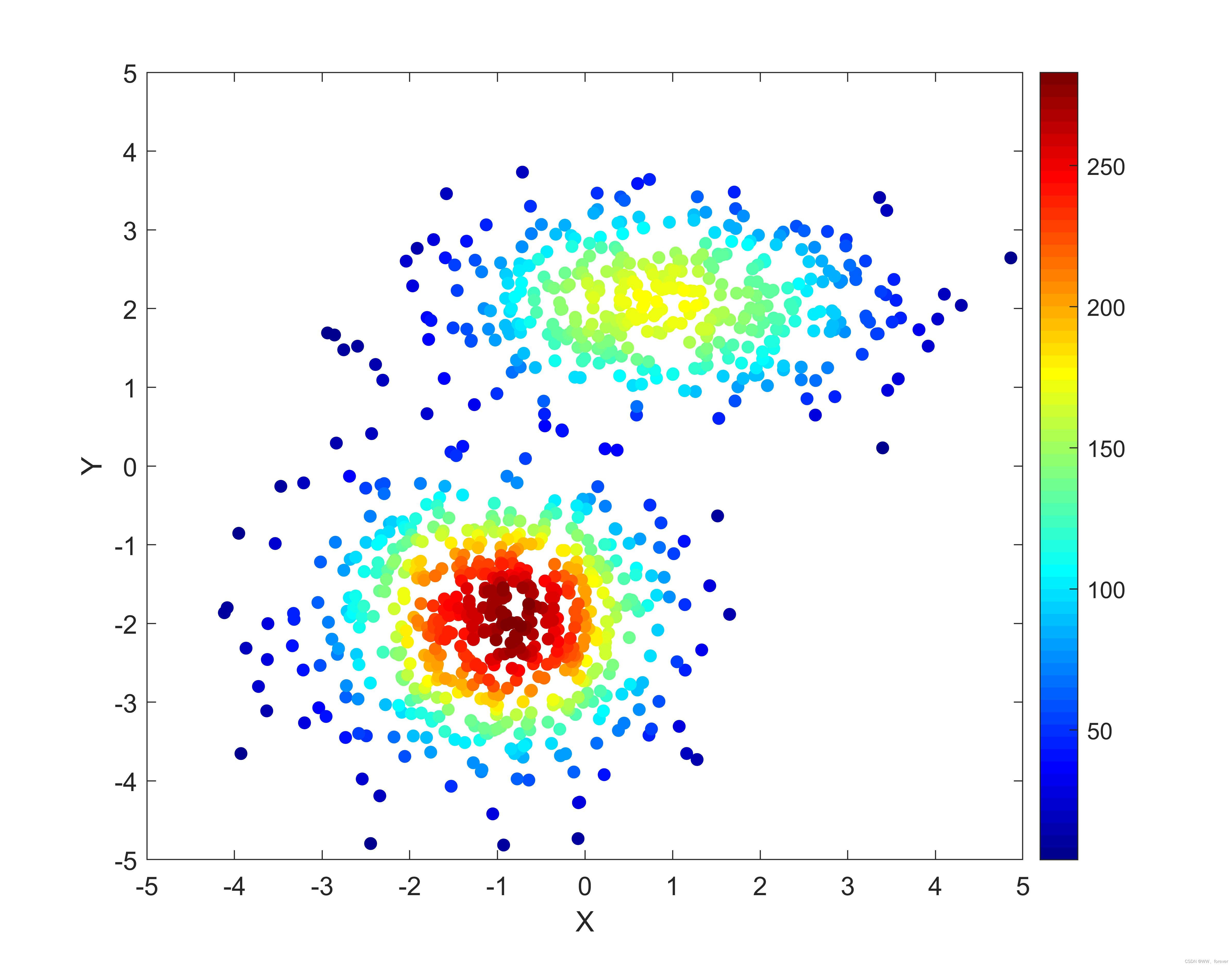
h(1) = scatter(XYZ(sortI, 1), XYZ(sortI, 2), [], XYZ(sortI, 3), 'filled');
colormap jet
xlabel("X");
ylabel("Y");
axis([axismin axismax axismin axismax]);
gc = get(gca);
set(gcf, 'position', [300, 100, Length, Width]);
set(gca,'fontsize',12);
colorbar

图形如下：

3 方法三：

3.1 案例

function []=scatter_plot_sta(x,y)
X =x;
Y =y;
numbins = 100;
    [values, centers] = hist3([X Y], [numbins numbins]);
    centers_X = centers{1,1};
    centers_Y = centers{1,2};
    binsize_X = abs(centers_X(2) - centers_X(1)) / 2;
    binsize_Y = abs(centers_Y(2) - centers_Y(1)) / 2;
    bins_X = zeros(numbins, 2);
    bins_Y = zeros(numbins, 2);
    for i = 1:numbins
        bins_X(i, 1) = centers_X(i) - binsize_X;
        bins_X(i, 2) = centers_X(i) + binsize_X;
        bins_Y(i, 1) = centers_Y(i) - binsize_Y;
        bins_Y(i, 2) = centers_Y(i) + binsize_Y;
    end
    scatter_COL = zeros(length(X), 1);
    onepercent = round(length(X) / 100);
    for i = 1:length(X)
        if (mod(i,onepercent) == 0)
            fprintf('.');
        end            
        last_lower_X = NaN;
        last_higher_X = NaN;
        id_X = NaN;
        c_X = X(i);
        last_lower_X = find(c_X >= bins_X(:,1));
        if (~isempty(last_lower_X))
            last_lower_X = last_lower_X(end);
        else
            last_higher_X = find(c_X <= bins_X(:,2));
            if (~isempty(last_higher_X))
                last_higher_X = last_higher_X(1);
            end
        end
        if (~isnan(last_lower_X))
            id_X = last_lower_X;
        else
            if (~isnan(last_higher_X))
                id_X = last_higher_X;
            end
        end
        last_lower_Y = NaN;
        last_higher_Y = NaN;
        id_Y = NaN;
        c_Y = Y(i);
        last_lower_Y = find(c_Y >= bins_Y(:,1));
        if (~isempty(last_lower_Y))
            last_lower_Y = last_lower_Y(end);
        else
            last_higher_Y = find(c_Y <= bins_Y(:,2));
            if (~isempty(last_higher_Y))
                last_higher_Y = last_higher_Y(1);
            end
        end
        if (~isnan(last_lower_Y))
            id_Y = last_lower_Y;
        else
            if (~isnan(last_higher_Y))
                id_Y = last_higher_Y;
            end
        end
        scatter_COL(i) = values(id_X, id_Y);
    end  
scatter(x, y, 50, scatter_COL, '.' );
colormap('jet');
h = colorbar;
caxis([0 10]);
% plot(x,y,'dk','MarkerSize',5,'MarkerFaceColor','k');
%  title('Product Comparison');
xlabel('ET FLDAS','FontSize',12,'FontWeight','normal','Color','k');
ylabel('ET MODIS','FontSize',12,'FontWeight','normal','Color','k');
 xlim([-1 4]);ylim([-1 4])
hold on
N=length(x);
a=polyfit(x,y,1);
C=corrcoef(x,y);
R=C(1,2)^2;
XX = x;
YY = y;
  nb_obs = length(XX);
    obs = XX;
    theo = YY;    
    sum_obs = sum(obs);  %%%%%%%%XX
  sum_theo = sum(theo);  %%%%%%%%%YY
  sum_sq_obs = sum(obs.^2);
  sum_sq_theo = sum(theo.^2);
  buf = theo - obs;  
  sum_diff = sum(buf);
  buf = buf.^2;  
  sum_sq_diff = sum(buf);
  buf = theo .* obs;
  cov = sum(buf);
  rse = sqrt(sum_sq_diff/(nb_obs - 2));
    bias = sum_diff./nb_obs;
  avg_obs = sum(obs)./nb_obs;
  avg_theo = sum(theo)./nb_obs;
  cov = (cov/nb_obs) - (avg_obs .* avg_theo);
  stdv_obs = sqrt((sum_sq_obs - (sum_obs.^2./nb_obs))./nb_obs);  
  stdv_theo = sqrt((sum_sq_theo - (sum_theo.^2./nb_obs))./nb_obs);
  slope_t1 = cov./stdv_obs.^2;
    intercept_t1 = avg_theo - (slope_t1.*avg_obs);
    rsq = (cov./(stdv_obs .* stdv_theo)).^2;   
    MRE = 100*((sum_obs - sum_theo)./sum_theo);   %% (Mod-Ins)/In    
    RE = MRE./nb_obs;     
    shi= abs(MRE)./nb_obs;    
    % Wenzhao edition on the biases calculation
A = XX./YY;
A2 = A(A~=0 & isfinite(A));
% Other way to exclude NAN and Inf: 
% B = A( ~any( isnan( A ) | isinf( A ), 2 ),: )
% ψ_i
ratio= A2 -1;
N=length(ratio);
bias = 100*sum(ratio)./N;
bias_abs = 100*sum(abs(ratio))./N;
% MaxSP=max(x);MaxV=max(y);Maxi=1.1*max(MaxSP,MaxV);
Maxi= 2000;
ax=linspace(0,Maxi,2000);
plot(ax,10*ax,'k');hold on
axis([0 4 0 4])
set(gca,'FontSize',12)
%set(gca,'XTick',(0:10:150))
title('BSk')
axis square
text(1*Maxi/500,9.0*Maxi/10,['N = ',num2str(N)], 'FontSize',12)
text(1*Maxi/500,8.25*Maxi/10,['R^2 = ',num2str(round(1000*R)/1000)], 'FontSize',12)
text(1*Maxi/500,7.50*Maxi/10,['RMSE = ',num2str(round(1000*rse)/1000)], 'FontSize',12)
text(1*Maxi/500,6.75*Maxi/10,['\Psi= ',num2str(round(1000*bias)/1000),' %'], 'FontSize',12)
text(1*Maxi/500,6.0*Maxi/10,['|\Psi|= ',num2str(round(1000*bias_abs)/1000),' %'], 'FontSize',12)
ay=a(1)*ax+a(2);%a=round(100*a)/100;disp(a)
plot(ax,ay,'r')
RegrssStr=['Y = ',num2str(round(a(1),2)),'*X +',num2str(round(a(2),2))];
%%% xlim([0 0.08]);ylim([0 0.08])
legend({'Data points','Y = 10*X',RegrssStr},'Location','northeast','FontSize',12);
box on
set(gca,'LineWidth',1.2)

参考

1.代码参考Matlab绘制卫星降雨散点密度图
2.博客-Matlab绘制散点密度图
3.博客-MATLAB实例：散点密度图
4.scatplot函数-scatplot