从头构建神经网络

从头构建神经网络

Building a neural network from sractch
仅用numpy实现神经网络，并用于实际的回归预测任务

---

I 数据集

数据集来源国家统计局

注：
　　　1.铁路运输数据来源于中国国家铁路集团有限公司、公路水路运输数据来源于交通运输部，民航运输数据来源于中国民用航空局。
　　　2.自2020年1月起，交通运输部根据2019道路货物运输量专项调查调整月度公路货物运输量、公路货物运输周转量统计口径，同比增速按照调整后可比口径计算。
　　　3.自2020年1月起，水路运输（海洋）统计方式改变，由行业主管部门报送调整为企业联网直报，2020年以可比口径计算增速。
　　　4.从2015年1月起，铁路客运统计口径发生变化，由按售票数统计改为按乘车人数统计。
　　　5.根据2013年开展的交通运输业经济统计专项调查，我部对公路水路运输量的统计口径和推算方案进行了调整。有关2014年月度公路水路客货运输量均按新方案推算并进行更新。
数据来源：国家统计局

数据集读取

import numpy as np
import pandas as pd
from sklearn.utils import resample

data = pd.read_csv('国家统计局月度数据统计.csv',encoding='gbk')
print('Shape:',data.shape)
data.head()

划分X和Y，我们的目的就是希望训练一个神经网络来通过上图data各列数据去预测客运量当期值(万人)，回归预测。

具体而言，通过2013年1月的所有数据（一整行）去预测2013年2月的客运量当期值(万人)，通过2013年2月的所有数据（一整行）去预测2013年3月的客运量当期值(万人).

# 空值填充
data.fillna(0,inplace=True)

num_columns = [i for i in data.columns if i not in ['时间']]
X_ = data[num_columns].values[:-1]
Y_ = data['客运量当期值(万人)'].values[1:]


X_ = (X_ - np.mean(X_ , axis=0)) / np.std(X_ , axis = 0)
print(len(X_),len(Y_))
print('第一个Y为',Y_[0],'最后一个Y为',Y_[-1])

数据集部分不再阐述，让我们主要关注神经网络的构建。

II 神经网络构建

2.1 构建基类

首先让我们明确神经网络中应该有的模块及功能：

1. Forward:前向传播 Funtion , how to calculate the inputs
2. Backforward:反向传播BP Funtion , how to get the gredients when backprogramming
3. Gradient:梯度“下降” Mapper ,the gradient map the this node of its inputs node
4. Inputs:输入 List, the input nodes of this node
5. Outputs:输出 List , the output node of this node

2.1.1 Node

简单来说每个节点的作用是这样的：
$$Input->Linear->Activation$$
通俗理解就是
$$(x->k\ast x+b->sigmoid)$$

因为在神经网络中又包含函数、字典、列表这些共同特性，让我们用面向对象的方式来组织这个框架

构建基类代码实现如下

class Node:
    """
    Each node in neural networks will have these attributes and methods
    """
    def __init__(self,inputs=[]):
        """
        if the node is operator of "ax + b" , the inputs will be x node , and the outputs
        of this is its successors , and the value is *ax + b*
        """
        self.inputs = inputs 
        self.outputs = []
        self.value = None
        self.gradients = { }
        
        for node in self.inputs:
            node.outputs.append(self) # bulid a connection relationship
            
    def forward(self):
        """Forward propogation
        
        compute the output value based on input nodes and store the value
        into *self.value*
        
        """
        # 虚类
        # 如果一个对象是它的子类，就必须要重新实现这个方法
        raise NotImplemented
        
    def backward(self):
        """Backward propogation
        
        compute the gradient of each input node and store the value
        into *self.gradients*
        
        """
        # 虚类
        # 如果一个对象是它的子类，就必须要重新实现这个方法       
        raise NotImplemented

2.1.2 Input

神经网络的输入节点定义如下，对于每个输入节点，都有两个属性：

1. forward：前向传播计算值
2. backward：反向传播，更新参数

class Input(Node):
    def __init__(self, name=''):
        Node.__init__(self, inputs=[])
        self.name = name
    
    def forward(self, value=None):
        if value is not None:
            self.value = value
        
    def backward(self):
        self.gradients = {}
        
        for n in self.outputs:
            grad_cost = n.gradients[self]
            self.gradients[self] = grad_cost
    
    def __repr__(self):
        return 'Input Node: {}'.format(self.name)

2.1.3 Linear

神经网络中的线性层如下
对于线性层，我们定义了 “wx+b”的前向计算，和反向传播时需要的对w、x、b参数的梯度值

class Linear(Node):
    def __init__(self, nodes, weights, bias):
        self.w_node = weights
        self.x_node = nodes
        self.b_node = bias
        Node.__init__(self, inputs=[nodes, weights, bias])
    
    def forward(self): 
        """compute the wx + b using numpy"""
        self.value = np.dot(self.x_node.value, self.w_node.value) + self.b_node.value
        
    
    def backward(self):
        
        for node in self.outputs:
            #gradient_of_loss_of_this_output_node = node.gradient[self]
            grad_cost = node.gradients[self]
            
            self.gradients[self.w_node] = np.dot(self.x_node.value.T, grad_cost) # loss对w的偏导 = loss对self的偏导 * self对w的偏导
            self.gradients[self.b_node] = np.sum(grad_cost * 1, axis=0, keepdims=False)
            self.gradients[self.x_node] = np.dot(grad_cost, self.w_node.value.T)

2.1.4 Sigmoid

神经网络中的激活函数如下，数学定义式，不再阐述

class Sigmoid(Node):
    def __init__(self, node):
        Node.__init__(self, [node])
        self.x_node = node
    
    def _sigmoid(self, x):
        return 1. / (1 + np.exp(-1 * x))
    
    def forward(self):
        self.value = self._sigmoid(self.x_node.value)
    
    def backward(self):
        y = self.value
        
        self.partial = y * (1 - y)
        
        for n in self.outputs:
            grad_cost = n.gradients[self]
            self.gradients[self.x_node] = grad_cost * self.partial

2.1.5 MSE

神经网络中的损失函数MSE定义，数学定义式，不再阐述

class MSE(Node):
    def __init__(self, y_true, y_hat):
        self.y_true_node = y_true
        self.y_hat_node = y_hat
        Node.__init__(self, inputs=[y_true, y_hat])
    
    def forward(self):
        y_true_flatten = self.y_true_node.value.reshape(-1, 1)
        y_hat_flatten = self.y_hat_node.value.reshape(-1, 1)
        
        self.diff = y_true_flatten - y_hat_flatten
        
        self.value = np.mean(self.diff**2)
        
    def backward(self):
        n = self.y_hat_node.value.shape[0]
        
        self.gradients[self.y_true_node] = (2 / n) * self.diff
        self.gradients[self.y_hat_node] =  (-2 / n) * self.diff

2.2 构建图

有关拓扑图的定义如下，在此你只需知道拓扑排序将神经网络中的各个节点进行有序排序，设定其有效的入度和出度。

def topological_sort(data_with_value):
    feed_dict = data_with_value 
    input_nodes = [n for n in feed_dict.keys()]

    G = {}
    nodes = [n for n in input_nodes]
    while len(nodes) > 0:
        n = nodes.pop(0)
        if n not in G:
            G[n] = {'in': set(), 'out': set()}
        for m in n.outputs:
            if m not in G:
                G[m] = {'in': set(), 'out': set()}
            G[n]['out'].add(m)
            G[m]['in'].add(n)
            nodes.append(m)

    L = []
    S = set(input_nodes)
    while len(S) > 0:
        n = S.pop()

        if isinstance(n, Input):
            n.value = feed_dict[n]
            ## if n is Input Node, set n'value as 
            ## feed_dict[n]
            ## else, n's value is caculate as its
            ## inbounds

        L.append(n)
        for m in n.outputs:
            G[n]['out'].remove(m)
            G[m]['in'].remove(n)
            # if no other incoming edges add to S
            if len(G[m]['in']) == 0:
                S.add(m)
    return L

def training_one_batch(topological_sorted_graph):
    # graph 是经过拓扑排序之后的 一个list
    for node in topological_sorted_graph:
        node.forward()
        
    for node in topological_sorted_graph[::-1]:
        node.backward()

def sgd_update(trainable_nodes, learning_rate=1e-2):
    for t in trainable_nodes:
        t.value += -1 * learning_rate * t.gradients[t]

def run(dictionary):
    return topological_sort(dictionary)

接下来，让我们定义神经网络每层的权重、输入输出，我们只设置了两个线性层

n_features = X_.shape[1]
n_hidden = 10
n_hidden_2 = 10

W1_ = np.random.randn(n_features , n_hidden)
b1_ = np.zeros(n_hidden)
W2_ = np.random.randn(n_hidden,1)
b2_ = np.zeros(1)

X, Y = Input(name='X'), Input(name='y')  # tensorflow -> placeholder
W1, b1 = Input(name='W1'), Input(name='b1')
W2, b2 = Input(name='W2'), Input(name='b2')

接下来，让我们定义神经网络的层

linear_output = Linear(X, W1, b1)
sigmoid_output = Sigmoid(linear_output)
Yhat = Linear(sigmoid_output, W2, b2)
loss = MSE(Y, Yhat)

让我们看一下我们输入输出经过拓扑排序后得到的神经网络图

input_node_with_value = { # -> feed_dict
    X:X_,
    Y:Y_,
    W1:W1_,
    W2:W2_,
    b1:b1_,
    b2:b2_
}
graph = topological_sort(input_node_with_value)
graph

III 训练

losses = []
epochs = 50000

batch_size = 64
steps_per_epoch = X_.shape[0] // batch_size
learning_rate = 0.1

for i in range(epochs):
    loss = 0
    
    for batch in range(steps_per_epoch):

        X_batch, Y_batch = resample(X_, Y_, n_samples=batch_size)
        
        X.value = X_batch
        Y.value = Y_batch
        
        
        training_one_batch(graph)
        sgd_update(trainable_nodes=[W1, W2, b1, b2], learning_rate=learning_rate)
        
        loss += graph[-1].value
        
    if i % 100 == 0:
        print('Epoch: {}, loss = {:.3f}'.format(i+1, loss/steps_per_epoch))
        losses.append(loss)

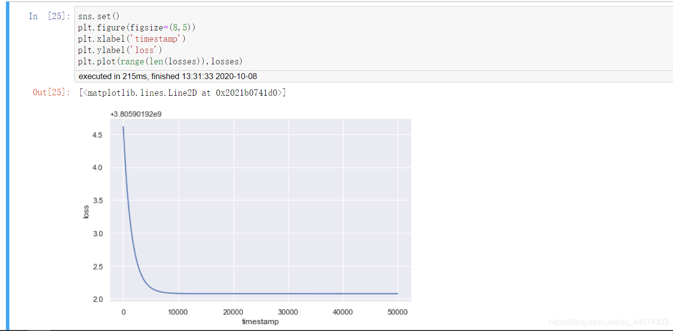
让我们看一下实现效果

import seaborn as sns
import matplotlib.pyplot as plt 
%matplotlib inline

sns.set()
plt.figure(figsize=(8,5))
plt.xlabel('timestamp')
plt.ylabel('loss')
plt.plot(range(len(losses)),losses)

仅用两个线性层即可实现如此的回归效果也还是可以的了，各位可以尝试通过增加线性层和激活函数来优化回归效果。

最后让我们看一下预测效果：


可以看出我们的预测效果还是可以接受的。
 
 
完整数据和代码文件请见Github：