线性回归应用（房价预测&餐厅经营预测）Python

预测特许餐厅经营利润

问题描述：

假设您是一家餐厅特许经营店的首席执行官，并且正在考虑在不同的城市开设一家新店。

• 您想将业务扩展到可能为您的餐厅带来更高利润的城市。

• 该连锁店已经在各个城市设有餐厅，并且您拥有来自城市的利润和人口数据。

• 您还拥有新餐厅候选城市的数据。

  • 对于这些城市，您有城市人口。

您能否使用这些数据来帮助您确定哪些城市可能会为您的企业带来更高的利润？

import numpy as np
import pandas as pd
import matplotlib.pyplot as plt
​
#计算损失函数
def compute_cost(X,Y,theta):
    theta=np.matrix(theta)
    cost=np.power(np.dot(X,(theta.T))-Y,2)
    return np.sum(cost)/(2*len(X))
​
#运行梯度下降算法
def compute_gradient(X,Y,theta,iters,alpha):
    theta=np.matrix(theta)
    m=X.shape[0]
    j=np.zeros((iters,1))
    for i in range(iters):
        h=np.dot(X,(theta.T))-Y
        temp=np.dot(h.T,X)
        theta=theta-alpha*temp/m
        j[i]=compute_cost(X,Y,theta)
    return theta,j
​
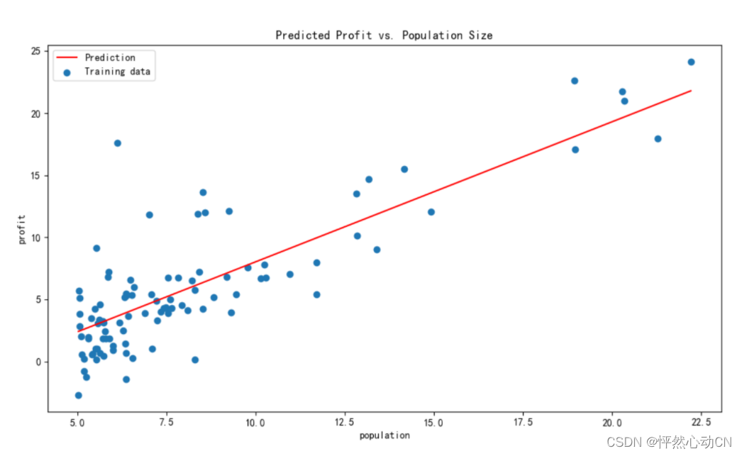
#决策边界，数据可视化
def drawFigure(data,theta):
    fig, ax = plt.subplots(figsize=(12, 8))
    x1=data['population']
    y1=data['profit']
    ax.scatter(x1,y1,label='Training data')
    x2=np.linspace(np.min(data['population']),np.max(data['population']),100)
    y2 = theta[0, 0] + theta[0, 1] * x2
    ax.plot(x2, y2, 'r', label='Prediction')
    ax.legend(loc=2)
    ax.set_xlabel('population')
    ax.set_ylabel('profit')
    ax.set_title("Predicted Profit vs. Population Size")
    plt.show()
​
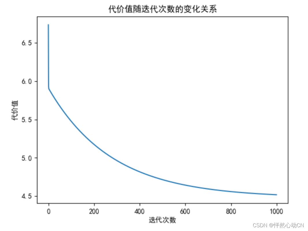
#代价值的变化曲线
def plotJ(j,iters):
    x=np.arange(0,iters)
    plt.plot(x,j)
    plt.xlabel("迭代次数")
    plt.ylabel("代价值")
    plt.title("代价值随迭代次数的变化关系")
    plt.show()
​
​
data=pd.read_csv("ex1data1.txt",delimiter=',',header=None,
                 names=['population','profit'])
x_train=data['population']
y_train=data['profit']
​
#初始化参数
data.insert(0,'ones',1)
alpha=0.001
#print(data.shape[1])结果为3，data.iloc为索引切片，前闭后开
loc=data.shape[1]
X=np.array(data.iloc[:,0:loc-1])
Y=np.array(data.iloc[:,loc-1:loc])
theta=np.zeros(X.shape[1])
X.shape,Y.shape,theta.shape
print(X.shape,Y.shape,theta.shape)
​
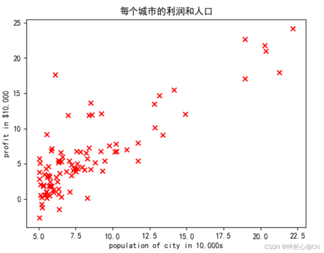
#可视化数据
plt.rcParams['font.sans-serif']=['SimHei']
plt.scatter(x_train,y_train,marker='x',c='r')
plt.title("每个城市的利润和人口")
plt.ylabel('profit in $10,000')
plt.xlabel('population of city in 10,000s')
plt.show()
​
theta,j=compute_gradient(X,Y,theta,iters=1000,alpha=0.01)
#print(theta)
#cost=compute_cost(X,Y,theta)
#print(cost)
plotJ(j,iters=1000)
drawFigure(data,theta)
print("请输入人口:")
a=float(input())
print(theta[0,0])
y=(theta[0,0]+theta[0,1]*a)*10000
print(y)

运行结果

 

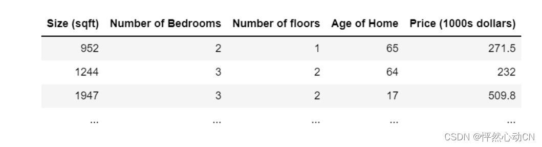
房价预测

问题描述：

As in the previous labs, you will use the motivating example of housing price prediction. The training data set contains many examples with 4 features (size, bedrooms, floors and age) shown in the table below. Note, in this lab, the Size feature is in sqft while earlier labs utilized 1000 sqft. This data set is larger than the previous lab.

We would like to build a linear regression model using these values so we can then predict the price for other houses - say, a house with 1200 sqft, 3 bedrooms, 1 floor, 40 years old.

数据集：

 

代码：

import numpy as np
import pandas as pd
from matplotlib import pyplot as plt
​
def linearRegression(alpha=0.01,iters=400):
    data=loadFile("houses.csv")
    X=np.array(data[:,0:-1])
    #转换成100*1的二维数组，防止后边计算出错
    y=np.array(data[:,-1]).reshape(-1,1)
    X,columnsMean,columnStd=meanNormalization(X)
    pltMeanNormalization(X)
    #对均值归一化的结果在第一列插入1，放在第一列,前一个参数是插入的矩阵的形状
    X=np.hstack((np.ones((len(X),1)),X))
    #着重考虑theta
    num_theta=X.shape[1]
    theta=np.zeros((num_theta,1))
    thetas,j=gradientDescent(X,y,theta,alpha,iters)
    plotJ(j,iters)
    thetas=thetas.flatten()
    a=float(input("请输入参数:"))
    b = float(input("请输入参数:"))
    c = float(input("请输入参数:"))
    d = float(input("请输入参数:"))
   # price=thetas[0,0]+thetas[0,1]*X[:,1]+thetas[0,2]*X[:,2]+thetas[0,3]*X[:,3]+thetas[0,4]*X[:,4]
    price = thetas[0, 0] + thetas[0, 1] * (a-columnsMean[0])/columnStd[0] + thetas[0, 2] *(b-columnsMean[1])/columnStd[1
    ] + thetas[0, 3] * (c-columnsMean[2])/columnStd[2] + thetas[0, 4] * (d-columnsMean[3])/columnStd[3]
    print(price)
#读取数据
def loadFile(path):
    return np.loadtxt(path,delimiter=',',dtype=np.float64)
​
#均值归一化/特征值缩放
# mean()函数的功能是求取平均值，经常操作的参数是axis，以m*n的矩阵为例：
# axis不设置值，对m*n个数求平均值，返回一个实数
# axis = 0：压缩行，对各列求均值，返回1*n的矩阵
# axis = 1: 压缩列，对各行求均值，返回m*1的矩阵
​
def meanNormalization(X):
    columnsMean=np.mean(X,0)
    columnStd=np.std(X,0)
    for i in range(X.shape[1]):
        X[:,i]=(X[:,i]-columnsMean[i])/columnStd[i]
    return X,columnsMean,columnStd
​
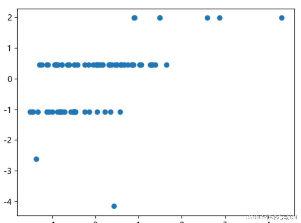
def pltMeanNormalization(X):
    plt.scatter(X[:,0],X[:,1])
    plt.show()
​
#损失函数
def costFunction(X,theta,y):
    m=len(X)
    j=np.sum(np.power(np.dot(X,theta)-y,2))/2*m
    return j
​
#梯度下降
def gradientDescent(X,y,theta,alpha,iters):
    m=len(X)
    theta=np.matrix(theta)
    j=np.zeros((iters,1))
    for i in range(iters):
        h=np.dot(X,theta)-y
        temp=np.dot((X.T),h)
        theta=theta-alpha*temp/m
        j[i]=costFunction(X,theta,y)
    thetas=theta
    return thetas,j
​
#代价值的变化曲线
def plotJ(j,iters):
    x=np.arange(0,iters)
    plt.plot(x,j)
    plt.xlabel("迭代次数")
    plt.ylabel("代价值")
    plt.title("代价值随迭代次数的变化关系")
    plt.show()
​
# 中文乱码解决方法
plt.rcParams['font.family'] = ['Arial Unicode MS','Microsoft YaHei','SimHei','sans-serif']
plt.rcParams['axes.unicode_minus'] = False
linearRegression()
​

运行结果：