吴恩达机器学习 逻辑回归 作业（是否被录取） Python

问题描述

In this part of the exercise, you will build a logistic regression model to predict whether a student gets admitted into a university.（预测学生是否被大学录取）

Suppose that you are the administrator of a university department and you want to determine each applicant’s chance of admission based on their results on two exams.

• You have historical data from previous applicants that you can use as a training set for logistic regression.

• For each training example, you have the applicant’s scores on two exams and the admissions decision.

• Your task is to build a classification model that estimates an applicant’s probability of admission based on the scores from those two exams.

翻译

在练习的这一部分中，您将构建一个逻辑回归模型来预测学生是否被大学录取。

假设您是大学部门的管理员，并且您想根据每个申请人在两次考试中的成绩来确定他们的录取机会。

• 您有以前申请人的历史数据，可以将其用作逻辑回归的训练集。

• 对于每个培训示例，您都有申请人在两次考试中的分数和录取决定。

• 您的任务是构建一个分类模型，该模型根据这两项考试的分数估计申请人的录取概率。

代码结构

 

代码

import numpy as np
import pandas as pd
from matplotlib import pyplot as plt

def LogistqRegression(alpha=0.001,iters=100000):
    data=readTxt(r"C:\Users\admin-zq\Documents\2022-Machine-Learning-Specialization-main\Supervised Machine Learning_ Regression and Classification\week3\9.Week 3 practice lab logistic regression\data\ex2data1.txt")
    dataPosition(data)
    X,Y,theta=readyData(data)
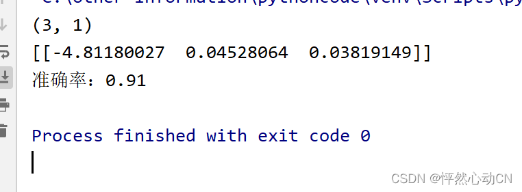
    theta=theta.reshape(-1,1)
    print(theta.shape)
    thetas,j=gradient(X,Y,alpha,iters,theta)
    thetas=thetas.flatten()
    print(thetas)
    plotJ(j,iters)
    boundary(thetas,data)
    predictions=predict(thetas,X)
    correct=[1 if a==b else 0 for (a,b) in zip(predictions,Y)]
    accuracy=sum(correct)/len(X)
    print('准确率：{}'.format(accuracy))
    # boundary(thetas,data)

#读取数据
def readTxt(path):
    return pd.read_csv(path,delimiter=',',header=None,names=['exam1','exam2','IsAdmited'])

#数据预处理
def readyData(data):
    data.insert(0,'ones',1)
    loc=data.shape[1]
    X=np.array(data.iloc[:,0:loc-1])
    Y=np.array(data.iloc[:,loc-1:loc])
    theta=np.zeros(X.shape[1])
    return X,Y,theta

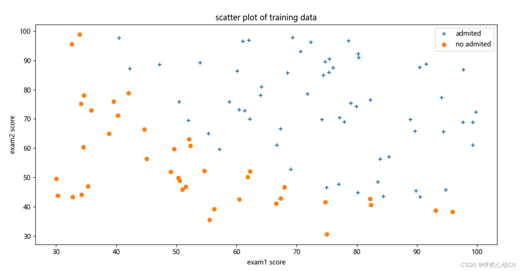
#查看数据分布
def dataPosition(data):
    AdmitedData=data[data['IsAdmited'].isin([1])]
    noAdmitedData=data[data['IsAdmited'].isin([0])]
    fig,ax=plt.subplots(figsize=(12,8))
    ax.scatter(AdmitedData['exam1'],AdmitedData['exam2'],marker='+',label='admited')
    ax.scatter(noAdmitedData['exam1'],noAdmitedData['exam2'],marker='o',label='no admited')
    ax.legend(loc=1)
    ax.set_xlabel('exam1 score')
    ax.set_ylabel('exam2 score')
    ax.set_title("scatter plot of training data")
    plt.show()

#sigmoid函数
def Sigmoid(z):
   return 1/(1+np.exp(-z))

#损失函数
def computeCost(X,Y,theta):
    theta=np.matrix(theta)
    h=Sigmoid(np.dot(X,theta))
    a=np.multiply((-Y),np.log(h))
    b=np.multiply((1-Y),np.log(1-h))
    j=np.sum(a-b)/len(X)
    return j

#梯度下降
def gradient(X,Y,alpha,iters,theta):
    m=len(X)
    num_theta=len(theta)
    temp_theta=np.matrix(np.zeros((num_theta,iters)))
    j = np.zeros((iters, 1))
    for i in range(iters):
        hypothesis=Sigmoid(np.dot(X,theta))
        temp_theta[:,i]=theta-(alpha/m)*(np.dot(np.transpose(X),(hypothesis-Y)))
        theta=temp_theta[:,i]
        j[i]=computeCost(X,Y,theta)
    thetas=theta
    return thetas,j

#代价值的变化曲线
def plotJ(j,iters):
    x=np.arange(0,iters)
    plt.plot(x,j)
    plt.xlabel("迭代次数")
    plt.ylabel("代价值")
    plt.title("代价值随迭代次数的变化关系")
    plt.show()

# 模型预测
def predict(theta,X):
    theta=np.matrix(theta)
    temp=Sigmoid(X*theta.T)
    return [1 if x>=0.5 else 0 for x in temp]

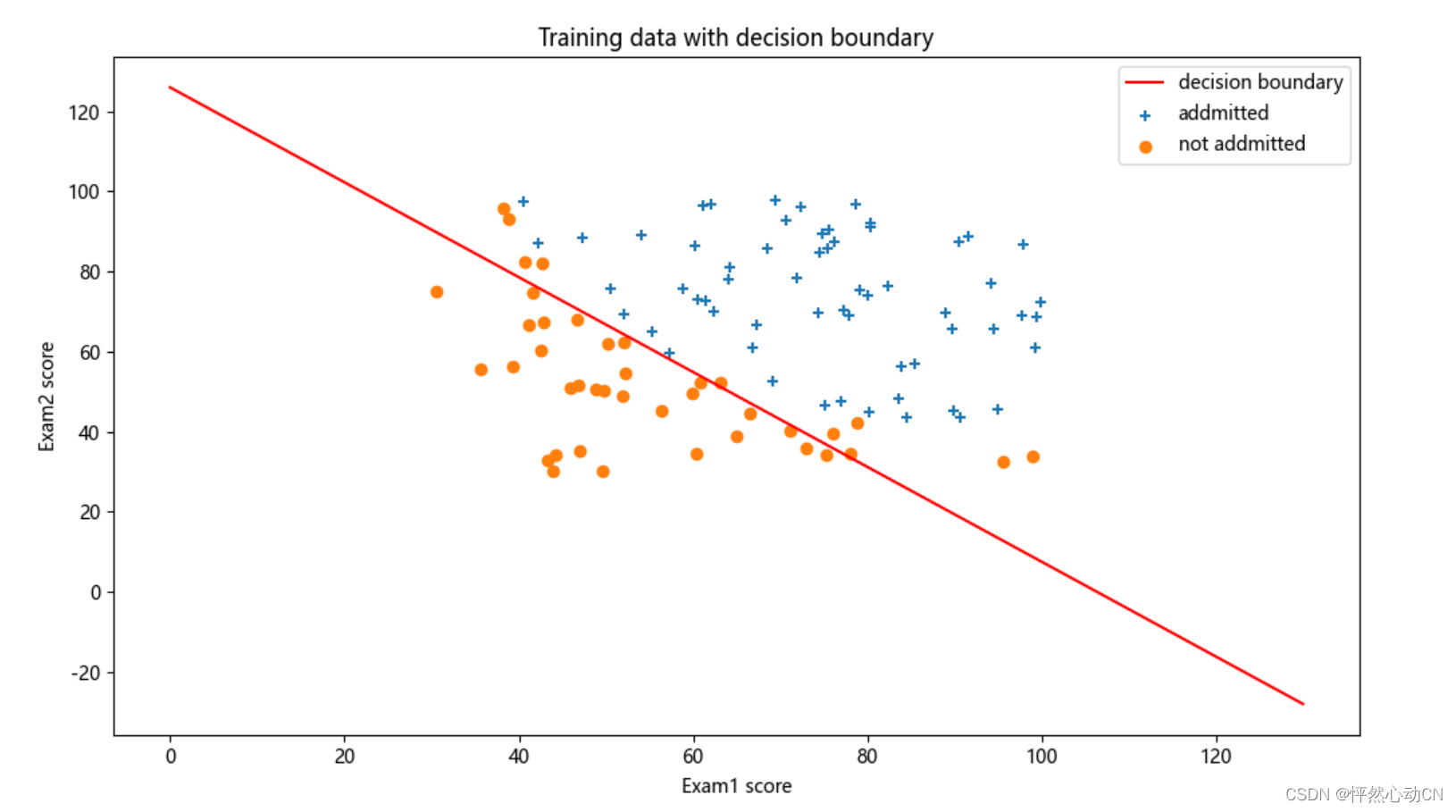
#决策边界
def decision(x1,theta):
    return [(-theta[0,0] - theta[0,1] * x1) / theta[0,2]]
#画出决策边界
def boundary(theta,data):
    # 决策边界，数据可视化

    admittedData = data[data['IsAdmited'].isin([1])]
    noAdmittedData = data[data['IsAdmited'].isin([0])]
    fig, ax = plt.subplots(figsize=(12, 8))
    ax.scatter(admittedData['exam1'], admittedData['exam2'], marker='+', label='addmitted')
    ax.scatter(noAdmittedData['exam2'], noAdmittedData['exam1'], marker='o', label="not addmitted")
    x1 = np.arange(130,step=0.1)
    x2 =-(theta[0,0] + theta[0,1] * x1) / theta[0,2]
    ax.plot(x1, x2, color='r', label="decision boundary")
    ax.legend(loc=1)
    ax.set_xlabel('Exam1 score')
    ax.set_ylabel('Exam2 score')
    ax.set_title("Training data with decision boundary")
    plt.show()


# 中文乱码解决方法
plt.rcParams['font.family'] = ['Arial Unicode MS','Microsoft YaHei','SimHei','sans-serif']
plt.rcParams['axes.unicode_minus'] = False
LogistqRegression()

运行结果