


数据分析
数据统计与计算
本节讨论使用Pandas来对数据进行处理和分析,主要包括以下内容
- 获取数据的统计信息
- 显示数据类型
转换数据类型 - 去除数据的重复值
- 对数据进行分组
- 寻找数据间的关系
- 计算百分比
在上一节“数据读取”中,我们用到了Pandas。现在我们将更深入了解Pandas在处理数据方面的应用。
首先先复习一下上节课中用Pandas读取CSV文件的代码:
import pandas as pd

# 创建列名列表
names = ['age', 'workclass', 'fnlwgt', 'education', 'educationnum', 'maritalstatus', 'occupation', 'relationship', 'race',
        'sex', 'capitalgain', 'capitalloss', 'hoursperweek', 'nativecountry', 'label']
# 利用定义好的列名来读取数据
df = pd.read_csv("data/adult.data", header=None, names=names)

print(df.head())
获取数据的统计信息
首先我们使用Pandas的函数来查看数据,以更好地了解数据可能存在的问题。Describe()函数将为我们提供计数和一些连续变量的统计信息。
import pandas as pd
names = ['age', 'workclass', 'fnlwgt', 'education', 'educationnum', 'maritalstatus', 'occupation', 'relationship', 'race',
        'sex', 'capitalgain', 'capitalloss', 'hoursperweek', 'nativecountry', 'label']
train_df = pd.read_csv("adult.data", header=None, names=names)
print(train_df.describe())
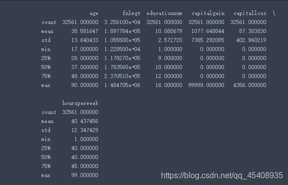
在得到的结果中,有mean,std,min,max,和一些不同百分比。
注意:请记住,异常值比中值对平均值的影响更大。另外,我们可以对标准差进行平方以获得方差。
我们可以发现结果中并没有包含所有列,那是因为describe()函数只对数值型的列进行统计。
显示数据类型
我们可以用info()函数来查看数据的类型
import pandas as pd

# 读取数据
names = ['age', 'workclass', 'fnlwgt', 'education', 'educationnum', 'maritalstatus', 'occupation', 'relationship', 'race',
        'sex', 'capitalgain', 'capitalloss', 'hoursperweek', 'nativecountry', 'label']
train_df = pd.read_csv("adult.data", header=None, names=names)

print(train_df.info())  # 使用inf()函数
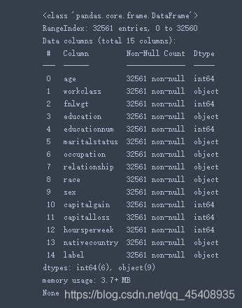
结果如图所示,在dataframe中有两种数据类型object和int64。我们可以把object类型当作字符串类型,把int64当作正数类型。
转换数据类型
如果说某一列数据的类型错误,我们可以用下面的函数进行转换:
- to_numeric()
- to_datetime()
- to_string()
例如:
df['numeric_column'] = pd.to_numeric(df['string_column'])
我们还可以从i上面使用info()函数获取的结果中查看每列非空值的计数以及数据的内存使用情况。
去除数据的重复值
另一个有用的步骤是查看列的都有哪些不重复的值。这是relationship列的示例:
import pandas as pd
names = ['age', 'workclass', 'fnlwgt', 'education', 'educationnum', 'maritalstatus', 'occupation', 'relationship', 'race',
        'sex', 'capitalgain', 'capitalloss', 'hoursperweek', 'nativecountry', 'label']
train_df = pd.read_csv("adult.data", header=None, names=names)
print(train_df['relationship'].unique())
输出:
[' Not-in-family' ' Husband' ' Wife' ' Own-child' ' Unmarried'
 ' Other-relative']
上面显示了relationship列都有哪些取值,并且我们可以统计每个值出现的次数:
import pandas as pd
names = ['age', 'workclass', 'fnlwgt', 'education', 'educationnum', 'maritalstatus', 'occupation', 'relationship', 'race',
        'sex', 'capitalgain', 'capitalloss', 'hoursperweek', 'nativecountry', 'label']
train_df = pd.read_csv("adult.data", header=None, names=names)
print(train_df['relationship'].value_counts())
输出:
 Husband           13193
 Not-in-family      8305
 Own-child          5068
 Unmarried          3446
 Wife               1568
 Other-relative      981
Name: relationship, dtype: int64
从输出结果可以看出,relationship列的所有取值,并且统计出了每个取值出现的次数。Husband出现的次数最多,Other-relative出现的次数最少。
对数据进行分组
python中groupby()函数主要的作用是进行数据的分组以及分组后的组内运算。groupby()需要传入要分组的列,然后再传入计算列,最后该函数会按组返回计算结果。如下示例:
import pandas as pd
names = ['age', 'workclass', 'fnlwgt', 'education', 'educationnum', 'maritalstatus', 'occupation', 'relationship', 'race',
        'sex', 'capitalgain', 'capitalloss', 'hoursperweek', 'nativecountry', 'label']
train_df = pd.read_csv("adult.data", header=None, names=names)

# 按relationship进行分组,然后对label列的统计值进行归一化 处理
print(train_df.groupby('relationship')['label'].value_counts(normalize=True))
输出:
relationship     label
 Husband          <=50K    0.551429
                  >50K     0.448571
 Not-in-family    <=50K    0.896930
                  >50K     0.103070
 Other-relative   <=50K    0.962283
                  >50K     0.037717
 Own-child        <=50K    0.986780
                  >50K     0.013220
 Unmarried        <=50K    0.936738
                  >50K     0.063262
 Wife             <=50K    0.524872
                  >50K     0.475128
Name: label, dtype: float64
上面我们所做的是按relationship变量分组,然后对label变量值计数。对于这些数据,label是收入是否大于50k。我们可以从上面看到55%的丈夫年收入超过5万。因为使用了normalize=True参数,所以我们收到了百分比。
我们还可以使用Pandas对组进行多种类型的计算。例如,在这里通过workclass字段我们可以看到的不同的workclass每周平均工作时间
import pandas as pd
names = ['age', 'workclass', 'fnlwgt', 'education', 'educationnum', 'maritalstatus', 'occupation', 'relationship', 'race',
        'sex', 'capitalgain', 'capitalloss', 'hoursperweek', 'nativecountry', 'label']
train_df = pd.read_csv("adult.data", header=None, names=names)
print(train_df.groupby(['workclass'])['hoursperweek'].mean())
输出:
workclass
 ?                   31.919390
 Federal-gov         41.379167
 Local-gov           40.982800
 Never-worked        28.428571
 Private             40.267096
 Self-emp-inc        48.818100
 Self-emp-not-inc    44.421881
 State-gov           39.031587
 Without-pay         32.714286
Name: hoursperweek, dtype: float64
从输出结果可以看出,Federal-gov 平均 Local-gov 工作更多。Never-worked 工作的平均时间约为28小时。
寻找数据间的关系
另一个有用的统计方法是相关性。如果需要复习相关性,请查阅Wikipedia。我们可以使用该corr函数计算dataFrame的所有成对相关性。
import pandas as pd
names = ['age', 'workclass', 'fnlwgt', 'education', 'educationnum', 'maritalstatus', 'occupation', 'relationship', 'race',
        'sex', 'capitalgain', 'capitalloss', 'hoursperweek', 'nativecountry', 'label']
train_df = pd.read_csv("adult.data", header=None, names=names)

# 计算相关性
print(train_df.corr())
输出:
                   age    fnlwgt  educationnum  capitalgain  capitalloss  \
age           1.000000 -0.076646      0.036527     0.077674     0.057775
fnlwgt       -0.076646  1.000000     -0.043195     0.000432    -0.010252
educationnum  0.036527 -0.043195      1.000000     0.122630     0.079923
capitalgain   0.077674  0.000432      0.122630     1.000000    -0.031615
capitalloss   0.057775 -0.010252      0.079923    -0.031615     1.000000
hoursperweek  0.068756 -0.018768      0.148123     0.078409     0.054256

              hoursperweek
age               0.068756
fnlwgt           -0.018768
educationnum      0.148123
capitalgain       0.078409
capitalloss       0.054256
hoursperweek      1.000000
我们可以很快地发现,与其他所有相关性相比,“hoursperweek”与“educationnum”之间具有更高的相关性,但并不是很高。我们可以发现,结果中没有包含label这列。了解各变量与label之间的关系将很有用,因此我们来考虑一下:
import pandas as pd
names = ['age', 'workclass', 'fnlwgt', 'education', 'educationnum', 'maritalstatus', 'occupation', 'relationship', 'race',
        'sex', 'capitalgain', 'capitalloss', 'hoursperweek', 'nativecountry', 'label']
train_df = pd.read_csv("adult.data", header=None, names=names)

# 将字符串列label转换为数值型,当>=50时为1,其他情况为0
train_df['label_int'] = train_df.label.apply(lambda x: ">" in x)
print(train_df.corr())
输出:
                   age    fnlwgt  educationnum  capitalgain  capitalloss  \
age           1.000000 -0.076646      0.036527     0.077674     0.057775
fnlwgt       -0.076646  1.000000     -0.043195     0.000432    -0.010252
educationnum  0.036527 -0.043195      1.000000     0.122630     0.079923
capitalgain   0.077674  0.000432      0.122630     1.000000    -0.031615
capitalloss   0.057775 -0.010252      0.079923    -0.031615     1.000000
hoursperweek  0.068756 -0.018768      0.148123     0.078409     0.054256
label_int     0.234037 -0.009463      0.335154     0.223329     0.150526

              hoursperweek  label_int
age               0.068756   0.234037
fnlwgt           -0.018768  -0.009463
educationnum      0.148123   0.335154
capitalgain       0.078409   0.223329
capitalloss       0.054256   0.150526
hoursperweek      1.000000   0.229689
label_int         0.229689   1.000000
label和educationnum似乎有一些良好的相关性。不过要注意的一件事是,label是分类的,因此计算相关性实际上并没有应用,采用分组频率可能是一种更好的方法。
注意:分类变量是类别没有内在顺序的变量。例如性别。
另外,请记住,这些只是单变量相关性(在一个变量之间),并不考虑多变量效应(在多个变量之间)。我们还可以使用scipy具有p值优势的软件包来计算相关性。在“ Scipy”章节中对此进行了讨论。
计算百分比
最后让我们来看看Pandas提供的percentiles函数
import pandas as pd
names = ['age', 'workclass', 'fnlwgt', 'education', 'educationnum', 'maritalstatus', 'occupation', 'relationship', 'race',
        'sex', 'capitalgain', 'capitalloss', 'hoursperweek', 'nativecountry', 'label']
train_df = pd.read_csv("adult.data", header=None, names=names)

# Use the describe function to calculate the percentiles specified
print(train_df.describe(percentiles=[.01,.05,.95,.99]))
输出:
                age        fnlwgt  educationnum   capitalgain   capitalloss  \
count  32561.000000  3.256100e+04  32561.000000  32561.000000  32561.000000
mean      38.581647  1.897784e+05     10.080679   1077.648844     87.303830
std       13.640433  1.055500e+05      2.572720   7385.292085    402.960219
min       17.000000  1.228500e+04      1.000000      0.000000      0.000000
1%        17.000000  2.718580e+04      3.000000      0.000000      0.000000
5%        19.000000  3.946000e+04      5.000000      0.000000      0.000000
50%       37.000000  1.783560e+05     10.000000      0.000000      0.000000
95%       63.000000  3.796820e+05     14.000000   5013.000000      0.000000
99%       74.000000  5.100720e+05     16.000000  15024.000000   1980.000000
max       90.000000  1.484705e+06     16.000000  99999.000000   4356.000000

       hoursperweek
count  32561.000000
mean      40.437456
std       12.347429
min        1.000000
1%         8.000000
5%        18.000000
50%       40.000000
95%       60.000000
99%       80.000000
max       99.000000
重塑数据
本节说明了使用Pandas重塑和整理数据的方法。
包括以下内容:
- 数据透视表
- 交叉表
- 重塑
长到宽格式
宽到长格式
数据透视表
像Excel一样,我们可以使用pandas pivot_table功能来透视数据。为此,我们将使用该pivot_table()函数。
values参数是用于计算的列,index参数用于创建多个行的索引值,columns参数用于要在其上创建多个列的值。
您还可以使用aggfunc参数传递用于汇总数据透视表的函数
让我们看一个例子:
import numpy as np
import pandas as pd
names = ['age', 'workclass', 'fnlwgt', 'education', 'educationnum', 'maritalstatus', 'occupation', 'relationship', 'race',
        'sex', 'capitalgain', 'capitalloss', 'hoursperweek', 'nativecountry', 'label']
train_df = pd.read_csv("adult.data", header=None, names=names)

# 按label,relationship,workclass计算每周平均工作时间.
print(pd.pivot_table(train_df, values='hoursperweek', index=['relationship','workclass'],
               columns=['label'], aggfunc=np.mean).round(2))
输出:
label                               <=50K   >50K
relationship    workclass
 Husband         ?                  30.72  37.33
                 Federal-gov        42.34  43.05
                 Local-gov          41.40  44.56
                 Private            42.50  46.18
                 Self-emp-inc       48.29  50.49
                 Self-emp-not-inc   46.01  48.07
                 State-gov          38.67  45.17
                 Without-pay        34.25    NaN
 Not-in-family   ?                  31.29  39.44
                 Federal-gov        40.60  47.54
                 Local-gov          40.38  45.01
                 Never-worked       35.00    NaN
                 Private            40.20  47.03
                 Self-emp-inc       49.06  53.58
                 Self-emp-not-inc   41.53  45.02
                 State-gov          38.87  44.19
 Other-relative  ?                  29.10  40.00
                 Federal-gov        38.40  45.00
                 Local-gov          35.92  48.00
                 Private            37.44  40.74
                 Self-emp-inc       40.00  41.67
                 Self-emp-not-inc   36.16  49.29
                 State-gov          36.40  29.00
 Own-child       ?                  32.39  50.00
                 Federal-gov        35.11    NaN
                 Local-gov          35.59  41.25
                 Never-worked       24.80    NaN
                 Private            32.84  43.09
                 Self-emp-inc       39.60  43.75
                 Self-emp-not-inc   40.33  49.38
                 State-gov          30.10  38.33
                 Without-pay        35.00    NaN
 Unmarried       ?                  32.75  50.00
                 Federal-gov        39.30  43.65
                 Local-gov          40.09  45.79
                 Private            38.64  45.70
                 Self-emp-inc       45.74  58.11
                 Self-emp-not-inc   40.62  47.81
                 State-gov          38.15  44.56
                 Without-pay        37.50    NaN
 Wife            ?                  28.29  29.72
                 Federal-gov        38.93  39.74
                 Local-gov          37.87  40.38
                 Never-worked       40.00    NaN
                 Private            36.56  38.31
                 Self-emp-inc       44.67  38.14
                 Self-emp-not-inc   36.53  34.61
                 State-gov          36.50  39.10
                 Without-pay        23.67    NaN
对于给定的relationship,workclass和label,现在我们有每周的平均工作小时表。
交叉表
Crosstab是获取频数表的好方法。我们要做的是将两列传递给函数,您将获得这两个变量的所有成对组合的频数。
让我们看一个使用标签和关系作为我们的列的示例:
import numpy as np
import pandas as pd
names = ['age', 'workclass', 'fnlwgt', 'education', 'educationnum', 'maritalstatus', 'occupation', 'relationship', 'race',
        'sex', 'capitalgain', 'capitalloss', 'hoursperweek', 'nativecountry', 'label']
train_df = pd.read_csv("adult.data", header=None, names=names)

# 计算label and relationship之间的频数
print(pd.crosstab(train_df['label'], train_df.relationship))
输出:
relationship   Husband   Not-in-family   Other-relative   Own-child  \
label
 <=50K            7275            7449              944        5001
 >50K             5918             856               37          67

relationship   Unmarried   Wife
label
 <=50K              3228    823
 >50K                218    745
现在,我们已按label和relationship细分计数。第一个参数用于行,第二个参数用于列。我们还可以使用normalize=True参数对结果进行归一化。
import numpy as np
import pandas as pd
names = ['age', 'workclass', 'fnlwgt', 'education', 'educationnum', 'maritalstatus', 'occupation', 'relationship', 'race',
        'sex', 'capitalgain', 'capitalloss', 'hoursperweek', 'nativecountry', 'label']
train_df = pd.read_csv("adult.data", header=None, names=names)

# 具有标准化的表
print(pd.crosstab(train_df['label'], train_df.relationship, normalize=True))
输出:
relationship   Husband   Not-in-family   Other-relative   Own-child  \
label
 <=50K        0.223427        0.228771         0.028992    0.153589
 >50K         0.181751        0.026289         0.001136    0.002058

relationship   Unmarried      Wife
label
 <=50K          0.099137  0.025276
 >50K           0.006695  0.022880
重塑
借助Pandas,我们可以pivot()用来重塑数据。为了说明这个概念,我将使用来自个帖子代码以长格式创建一个dataframe。
import pandas.util.testing as tm; tm.N = 3
import numpy as np
import pandas as pd

def unpivot(frame):
    N, K = frame.shape
    data = {'value' : frame.values.ravel('F'),
            'variable' : np.asarray(frame.columns).repeat(N),
            'date' : np.tile(np.asarray(frame.index), K)}
    return pd.DataFrame(data, columns=['date', 'variable', 'value'])
df = unpivot(tm.makeTimeDataFrame())
print(df)
输出:
         date variable     value
0  2000-01-03        A  1.762265
1  2000-01-04        A -1.836282
2  2000-01-05        A  1.341377
3  2000-01-03        B -2.010261
4  2000-01-04        B -1.457658
5  2000-01-05        B  0.960505
6  2000-01-03        C  1.579438
7  2000-01-04        C  0.723217
8  2000-01-05        C -1.458282
9  2000-01-03        D -0.026408
10 2000-01-04        D  0.272848
11 2000-01-05        D -0.224588
在此示例中,variable的有A,B,Ç,这是一个长格式。为了使其具有更宽的格式,我们将创建列A,B和C并删除variable列
长格式到宽格式
这是我们将这种长格式转换为宽格式的方法:
import pandas.util.testing as tm; tm.N = 3
import numpy as np
import pandas as pd

def unpivot(frame):
    N, K = frame.shape
    data = {'value' : frame.values.ravel('F'),
            'variable' : np.asarray(frame.columns).repeat(N),
            'date' : np.tile(np.asarray(frame.index), K)}
    return pd.DataFrame(data, columns=['date', 'variable', 'value'])
df = unpivot(tm.makeTimeDataFrame())

# Use pivot to keep date as the index and value as the values, but use the vaiable column to create new columns
df_pivot = df.pivot(index='date', columns='variable', values='value')
print(df_pivot)
输出:
variable           A         B         C         D
date
2000-01-03 -0.579241  1.007006 -0.384546  0.491940
2000-01-04  0.470201 -0.645394 -0.564861 -0.395214
2000-01-05 -0.817290  0.554533  1.004388  1.702254
宽格式到长格式
为了将格式从宽转换为长,Pandas为我们提供了unstack()函数。
import pandas.util.testing as tm; tm.N = 3
import numpy as np
import pandas as pd

# 创建长格式数据
def unpivot(frame):
    N, K = frame.shape
    data = {'value' : frame.values.ravel('F'),
            'variable' : np.asarray(frame.columns).repeat(N),
            'date' : np.tile(np.asarray(frame.index), K)}
    return pd.DataFrame(data, columns=['date', 'variable', 'value'])
df = unpivot(tm.makeTimeDataFrame())

# 转为宽格式
df_pivot = df.pivot(index='date', columns='variable', values='value')

# 回到长格式
print(df_pivot.unstack())
输出:
variable  date
A         2000-01-03   -0.124403
          2000-01-04   -0.314589
          2000-01-05   -0.699477
B         2000-01-03   -0.896259
          2000-01-04   -0.301238
          2000-01-05    0.135009
C         2000-01-03   -1.981508
          2000-01-04   -0.119111
          2000-01-05   -3.041723
D         2000-01-03    0.348741
          2000-01-04   -0.937233
          2000-01-05    0.328904
dtype: float64


 4119
4119


 被折叠的 条评论
为什么被折叠?
被折叠的 条评论
为什么被折叠?
 到【灌水乐园】发言


