吴恩达机器学习2022-Jupyter-机器学习实例

KAY金

已于 2023-07-13 15:51:24 修改

阅读量1.6k

点赞数

分类专栏：机器学习文章标签：机器学习 jupyter 人工智能

于 2023-07-12 17:15:05 首次发布

本文链接：https://blog.csdn.net/qq_45605440/article/details/131685542

版权

机器学习专栏收录该内容

10 篇文章 5 订阅

订阅专栏

1 可选实验: 特征工程和多项式回归

1.1 目标

在这个实验室里:

探索特征工程和多项式回归，它可以让你使用线性回归机制来适应非常复杂，甚至非常非线性的函数。

1.2 工具

您将利用在以前的实验中开发的函数以及matplotlib和NumPy。

2 特征工程与多项式回归综述

线性回归提供了一种模型方法，公式形式为:

如果您的特性/数据是非线性的或者是特性的组合，该怎么办？例如，住房价格往往不与居住面积成线性关系，而是对小型或大型房屋造成上图所示曲线的惩罚。我们如何利用线性回归机制来适应这条曲线？回想一下，我们所拥有的“机制”是能够修改(1)中的参数 w，b，使方程“适合”训练数据。然而，(1)中 w，b 的任何调整都不会实现对非线性曲线的拟合。

2.1 多项式特征

上面我们考虑了一个数据是非线性的场景。让我们试着用我们目前所知道的来拟合一条非线性曲线。我们从一个简单的二次型开始: y = 1 + x^2。

# create target data
x = np.arange(0, 20, 1)
y = 1 + x**2
X = x.reshape(-1, 1)

model_w,model_b = run_gradient_descent_feng(X,y,iterations=1000, alpha = 1e-2)

plt.scatter(x, y, marker='x', c='r', label="Actual Value"); plt.title("no feature engineering")
plt.plot(x,X@model_w + model_b, label="Predicted Value");  plt.xlabel("X"); plt.ylabel("y"); plt.legend(); plt.show()

输出：

Iteration         0, Cost: 1.65756e+03
Iteration       100, Cost: 6.94549e+02
Iteration       200, Cost: 5.88475e+02
Iteration       300, Cost: 5.26414e+02
Iteration       400, Cost: 4.90103e+02
Iteration       500, Cost: 4.68858e+02
Iteration       600, Cost: 4.56428e+02
Iteration       700, Cost: 4.49155e+02
Iteration       800, Cost: 4.44900e+02
Iteration       900, Cost: 4.42411e+02
w,b found by gradient descent: w: [18.7], b: -52.0834

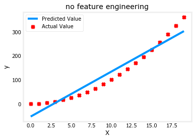
不出所料，不太合适。我们需要的是类似 y = w0x0^2 + b 或者多项式特征的东西。为此，您可以修改输入数据来设计所需的特性。如果将原始数据与平方 x 值的版本交换，则可以实现 y = w0·x0^2 + b。以 X * * 2交换 X 如下:

# create target data
x = np.arange(0, 20, 1)
y = 1 + x**2

# Engineer features 
X = x**2      #<-- added engineered feature

X = X.reshape(-1, 1)  #X should be a 2-D Matrix
model_w,model_b = run_gradient_descent_feng(X, y, iterations=10000, alpha = 1e-5)

plt.scatter(x, y, marker='x', c='r', label="Actual Value"); plt.title("Added x**2 feature")
plt.plot(x, np.dot(X,model_w) + model_b, label="Predicted Value"); plt.xlabel("x"); plt.ylabel("y"); plt.legend(); plt.show()

输出：

Iteration         0, Cost: 7.32922e+03
Iteration      1000, Cost: 2.24844e-01
Iteration      2000, Cost: 2.22795e-01
Iteration      3000, Cost: 2.20764e-01
Iteration      4000, Cost: 2.18752e-01
Iteration      5000, Cost: 2.16758e-01
Iteration      6000, Cost: 2.14782e-01
Iteration      7000, Cost: 2.12824e-01
Iteration      8000, Cost: 2.10884e-01
Iteration      9000, Cost: 2.08962e-01
w,b found by gradient descent: w: [1.], b: 0.0490

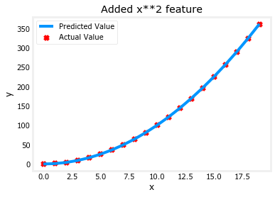
太好了！近乎完美。注意打印出来的 w 和 b 的值就在图表 w，b 的梯度下降法 w: [1. ]的右上方，b: 0.0490.梯度下降法修改了 w，b 的初始值为(1.0.0.049) ，或者 y = 1的模型为 * x20.0.049，非常接近我们的目标 y = 1 * x20 + 1。如果你运行的时间更长，可能会更匹配。

2.1.1 选择特征

上面，我们知道需要一个 x^2项。需要那些特征可能并不总是显而易见的。人们可以添加各种潜在的特性，以试图找到最有用的特性。例如，如果我们尝试: y = w0x0 + w1x1^2 + w2x3^2 + b。

# create target data
x = np.arange(0, 20, 1)
y = x**2

# engineer features .
X = np.c_[x, x**2, x**3]   #<-- added engineered feature

model_w,model_b = run_gradient_descent_feng(X, y, iterations=10000, alpha=1e-7)

plt.scatter(x, y, marker='x', c='r', label="Actual Value"); plt.title("x, x**2, x**3 features")
plt.plot(x, X@model_w + model_b, label="Predicted Value"); plt.xlabel("x"); plt.ylabel("y"); plt.legend(); plt.show()

输出：

Iteration         0, Cost: 1.14029e+03
Iteration      1000, Cost: 3.28539e+02
Iteration      2000, Cost: 2.80443e+02
Iteration      3000, Cost: 2.39389e+02
Iteration      4000, Cost: 2.04344e+02
Iteration      5000, Cost: 1.74430e+02
Iteration      6000, Cost: 1.48896e+02
Iteration      7000, Cost: 1.27100e+02
Iteration      8000, Cost: 1.08495e+02
Iteration      9000, Cost: 9.26132e+01
w,b found by gradient descent: w: [0.08 0.54 0.03], b: 0.0106

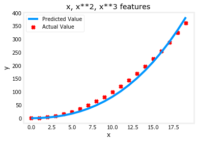
注意 w，[0.080.540.03]和 b 的值是0.0106。这意味着拟合/训练后的模型是:

0.08𝑥+0.54𝑥^2+0.03𝑥^3+0.0106。

梯度下降法强调了最适合 x^2数据的数据，即相对于其他数据增加 w1项。如果你要跑很长一段时间，它会继续减少其他术语的影响。梯度下降法是通过强调其相关参数来为我们选择“正确”的特征.

让我们回顾一下这个想法:

最初，这些特征被重新缩放，因此它们可以彼此比较

较小的权重值意味着较不重要/正确的特征，在极端情况下，当权重变为零或非常接近零时，相关的特征可用于将模型拟合到数据中。

以上，经过拟合，权值相关的 x^2特征要比 x 或 x^3的权重大得多，因为它在拟合数据时最有用。

2.1.2 另一种视角

根据目标数据的匹配程度选择多项式特征。另一种思考这个问题的方法是注意，一旦我们创建了新的特性，我们仍然在使用线性回归。考虑到这一点，最好的特征将是线性相对于目标。最好通过一个例子来理解这一点。

# create target data
x = np.arange(0, 20, 1)
y = x**2

# engineer features .
X = np.c_[x, x**2, x**3]   #<-- added engineered feature
X_features = ['x','x^2','x^3']

fig,ax=plt.subplots(1, 3, figsize=(12, 3), sharey=True)
for i in range(len(ax)):
    ax[i].scatter(X[:,i],y)
    ax[i].set_xlabel(X_features[i])
ax[0].set_ylabel("y")
plt.show()

输出：

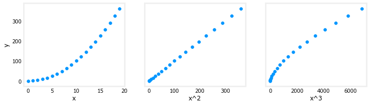
上面，很明显，x^2映射到目标值 y 的特征是线性的，线性回归可以很容易地使用该特征生成一个模型。

# create target data
x = np.arange(0,20,1)
X = np.c_[x, x**2, x**3]
print(f"Peak to Peak range by column in Raw        X:{np.ptp(X,axis=0)}")

# add mean_normalization 
X = zscore_normalize_features(X)     
print(f"Peak to Peak range by column in Normalized X:{np.ptp(X,axis=0)}")

输出：

Peak to Peak range by column in Raw        X:[  19  361 6859]
Peak to Peak range by column in Normalized X:[3.3  3.18 3.28]

现在，我们可以用更大的 alpha 值再试一次:

x = np.arange(0,20,1)
y = x**2

X = np.c_[x, x**2, x**3]
X = zscore_normalize_features(X) 

model_w, model_b = run_gradient_descent_feng(X, y, iterations=100000, alpha=1e-1)

plt.scatter(x, y, marker='x', c='r', label="Actual Value"); plt.title("Normalized x x**2, x**3 feature")
plt.plot(x,X@model_w + model_b, label="Predicted Value"); plt.xlabel("x"); plt.ylabel("y"); plt.legend(); plt.show()

输出：

Iteration         0, Cost: 9.42147e+03
Iteration     10000, Cost: 3.90938e-01
Iteration     20000, Cost: 2.78389e-02
Iteration     30000, Cost: 1.98242e-03
Iteration     40000, Cost: 1.41169e-04
Iteration     50000, Cost: 1.00527e-05
Iteration     60000, Cost: 7.15855e-07
Iteration     70000, Cost: 5.09763e-08
Iteration     80000, Cost: 3.63004e-09
Iteration     90000, Cost: 2.58497e-10
w,b found by gradient descent: w: [5.27e-05 1.13e+02 8.43e-05], b: 123.5000

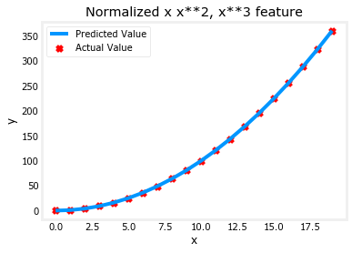
特性缩放使它更快地收敛。

再次注意 w 的值。W1项，也就是 x^2项是最重要的。梯度下降法几乎完全取消了 x^3这个术语。

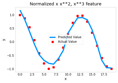
2.1.4 复杂函数

通过特征工程，即使是相当复杂的功能也可以被建模:

x = np.arange(0,20,1)
y = np.cos(x/2)

X = np.c_[x, x**2, x**3,x**4, x**5, x**6, x**7, x**8, x**9, x**10, x**11, x**12, x**13]
X = zscore_normalize_features(X) 

model_w,model_b = run_gradient_descent_feng(X, y, iterations=1000000, alpha = 1e-1)

plt.scatter(x, y, marker='x', c='r', label="Actual Value"); plt.title("Normalized x x**2, x**3 feature")
plt.plot(x,X@model_w + model_b, label="Predicted Value"); plt.xlabel("x"); plt.ylabel("y"); plt.legend(); plt.show()

输出：

Iteration         0, Cost: 2.24887e-01
Iteration    100000, Cost: 2.31061e-02
Iteration    200000, Cost: 1.83619e-02
Iteration    300000, Cost: 1.47950e-02
Iteration    400000, Cost: 1.21114e-02
Iteration    500000, Cost: 1.00914e-02
Iteration    600000, Cost: 8.57025e-03
Iteration    700000, Cost: 7.42385e-03
Iteration    800000, Cost: 6.55908e-03
Iteration    900000, Cost: 5.90594e-03
w,b found by gradient descent: w: [-1.61e+00 -1.01e+01  3.00e+01 -6.92e-01 -2.37e+01 -1.51e+01  2.09e+01
 -2.29e-03 -4.69e-03  5.51e-02  1.07e-01 -2.53e-02  6.49e-02], b: -0.0073