


example1
import matplotlib.pyplot as plt
import numpy as np
plt.rcParams['text.usetex'] = True
fig, ax = plt.subplots()
x = np.linspace(-10, 10)
ax.plot(x, x**2)
# adding table
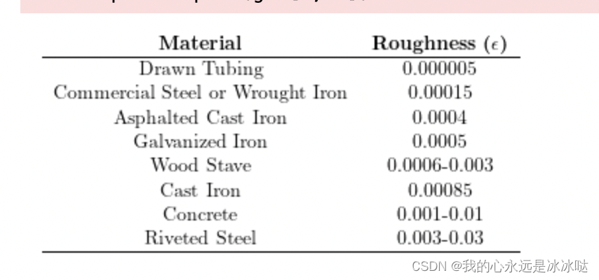
table = (r"\begin{tabular}{cc}"
r"\bf{Material} & \bf{Roughness ($\epsilon$)} \\"
r"\hline "
r"Drawn Tubing & 0.000005 \\"
r"Commercial Steel or Wrought Iron & 0.00015 \\"
r"Asphalted Cast Iron & 0.0004 \\"
r"Galvanized Iron & 0.0005 \\"
r"Wood Stave & 0.0006-0.003 \\"
r"Cast Iron & 0.00085 \\"
r"Concrete & 0.001-0.01 \\"
r"Riveted Steel & 0.003-0.03"
r"\end{tabular}")
ax.annotate(table, xy=(0, 60), ha='center', va='center')
plt.show()
结果如下
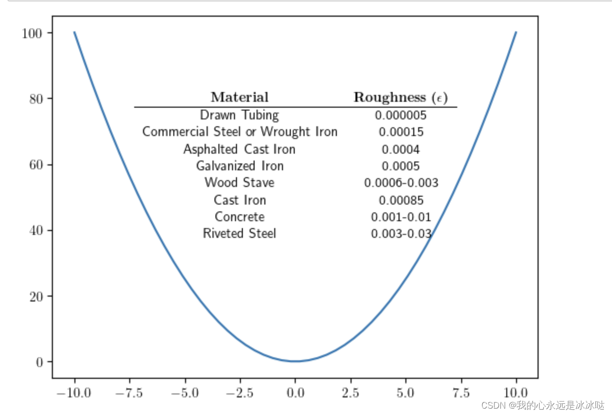
可以看到这个表格是显示的,
example2(三个图)
#!/usr/bin/env python3
# -*- coding: utf-8 -*-
"""
Created on Mon Oct  9 20:11:57 2017

@author: mraissi
"""

import numpy as np
import matplotlib as mpl
#mpl.use('pgf')

def figsize(scale, nplots = 1):
    fig_width_pt = 390.0                          # Get this from LaTeX using \the\textwidth
    inches_per_pt = 1.0/72.27                       # Convert pt to inch
    golden_mean = (np.sqrt(5.0)-1.0)/2.0            # Aesthetic ratio (you could change this)
    fig_width = fig_width_pt*inches_per_pt*scale    # width in inches
    fig_height = nplots*fig_width*golden_mean              # height in inches
    fig_size = [fig_width,fig_height]
    return fig_size

pgf_with_latex = {                      # setup matplotlib to use latex for output
    "pgf.texsystem": "xelatex",        # change this if using xetex or lautex
    "text.usetex": True,                # use LaTeX to write all text
    "font.family": "serif",
    "font.serif": [],                   # blank entries should cause plots to inherit fonts from the document
    "font.sans-serif": [],
    "font.monospace": [],
    "axes.labelsize": 10,               # LaTeX default is 10pt font.
    "font.size": 10,
    "legend.fontsize": 8,               # Make the legend/label fonts a little smaller
    "xtick.labelsize": 8,
    "ytick.labelsize": 8,
    "figure.figsize": figsize(1.0),     # default fig size of 0.9 textwidth
    "pgf.preamble": "\n".join([
        r"\usepackage[utf8x]{inputenc}",    # use utf8 fonts becasue your computer can handle it :)
        r"\usepackage[T1]{fontenc}",        # plots will be generated using this preamble
        ]),
    }
mpl.rcParams.update(pgf_with_latex)

import matplotlib.pyplot as plt

# I make my own newfig and savefig functions
def newfig(width, nplots = 1):
    fig = plt.figure(figsize=figsize(width, nplots))
    ax = fig.add_subplot(111)
    return fig, ax

def savefig(filename, crop = True):
    if crop == True:
#        plt.savefig('{}.pgf'.format(filename), bbox_inches='tight', pad_inches=0)
        plt.savefig('{}.pdf'.format(filename), bbox_inches='tight', pad_inches=0)
        plt.savefig('{}.eps'.format(filename), bbox_inches='tight', pad_inches=0)
    else:
#        plt.savefig('{}.pgf'.format(filename))
        plt.savefig('{}.pdf'.format(filename))
        plt.savefig('{}.eps'.format(filename))

## Simple plot
# fig, ax  = newfig(1.0)

# def ema(y, a):
#     s = []
#     s.append(y[0])
#     for t in range(1, len(y)):
#         s.append(a * y[t] + (1-a) * s[t-1])
#     return np.array(s)

# y = [0]*200
# y.extend([20]*(1000-len(y)))
# s = ema(y, 0.01)

# ax.plot(s)
# ax.set_xlabel('X Label')
# ax.set_ylabel('EMA')

# savefig('ema')
import numpy as np
import matplotlib.pyplot as plt
#from plotting import newfig, savefig
from mpl_toolkits.mplot3d import Axes3D
import matplotlib.gridspec as gridspec
from mpl_toolkits.axes_grid1 import make_axes_locatable
fig, ax = newfig(1.0, 1.5)
ax.axis('off')
gs0 = gridspec.GridSpec(1, 2)
gs0.update(top=1-0.06, bottom=1-1/3+0.05, left=0.15, right=0.85, wspace=0)
ax = plt.subplot(gs0[:, :])
# h = ax.imshow(Exact, interpolation='nearest', cmap='rainbow',
# extent=[t_star.min(),t_star.max(), lb[0], ub[0]],
# origin='lower', aspect='auto')
# divider = make_axes_locatable(ax)
# cax = divider.append_axes("right", size="5%", pad=0.05)
# fig.colorbar(h, cax=cax)
x = np.linspace(-2*np.pi, 2*np.pi)
y = np.sin(x)
ax.plot(x, y, '-', linewidth = 1.0)
ax.set_xlabel('$t$')
ax.set_ylabel('$x$')
ax.set_title('$u(t,x)$', fontsize = 10)
gs1 = gridspec.GridSpec(1, 2)
gs1.update(top=1-1/3-0.1, bottom=1-2/3, left=0.15, right=0.85, wspace=0.5)
ax = plt.subplot(gs1[0, 0])
#ax.plot(x_star,Exact[:,idx_t][:,None], 'b', linewidth = 2, label = 'Exact')
u0=np.cos(x)
ax.plot(x, u0, 'rx', linewidth = 2, label = 'Data')
ax.set_xlabel('$x$')
ax.set_ylabel('$u(t,x)$')
ax.set_title('$t = %.2f$\n%d trainng data' % (0.11, 150), fontsize = 10)
ax = plt.subplot(gs1[0, 1])
#ax.plot(x_star,Exact[:,idx_t + skip][:,None], 'b', linewidth = 2, label = 'Exact')
u1 = np.sin(x)+np.cos(x)
ax.plot(x, u1, 'rx', linewidth = 2, label = 'Data')
ax.set_xlabel('$x$')
ax.set_ylabel('$u(t,x)$')
ax.set_title('$t = %.2f$\n%d trainng data' % (0.2, 190), fontsize = 10)
ax.legend(loc='upper center', bbox_to_anchor=(-0.3, -0.3), ncol=2, frameon=False)
gs2 = gridspec.GridSpec(1, 2)
gs2.update(top=1-2/3-0.05, bottom=0, left=0.15, right=0.85, wspace=0.0)
ax = plt.subplot(gs2[0, 0])
ax.axis('off')
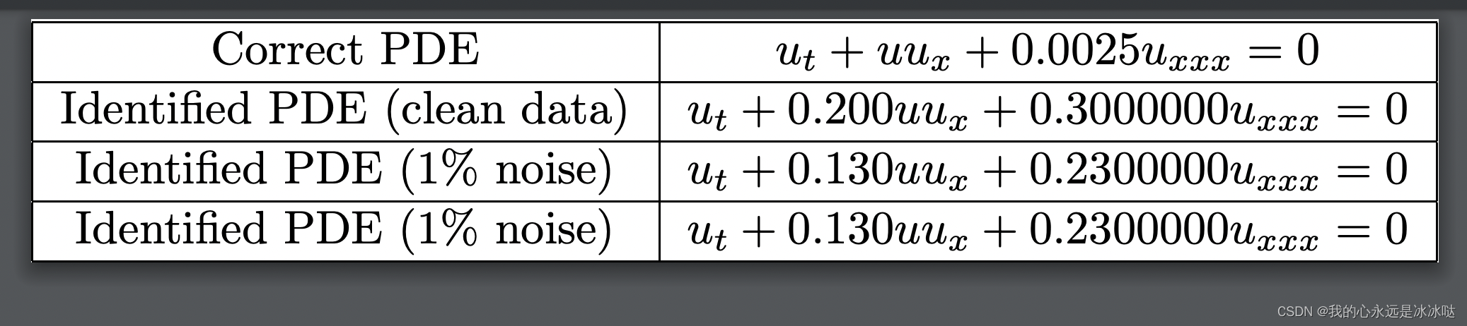
s1 = r'$\begin{tabular}{ |c|c| } \hline Correct PDE & $u_t + u u_x + 0.0025 u_{xxx} = 0$ \\ \hline Identified PDE (clean data) & '
s2 = r'$u_t + %.3f u u_x + %.7f u_{xxx} = 0$ \\ \hline ' % (0.2, 0.3)
s3 = r'Identified PDE (1\% noise) & '
s4 = r'$u_t + %.3f u u_x + %.7f u_{xxx} = 0$ \\ \hline ' % (0.13, 0.23)
s5 = r'\end{tabular}$'
s = s1+s2+s3+s4+s5
ax.text(-0.1,0.2,s)
savefig('./KdV')
结果如下
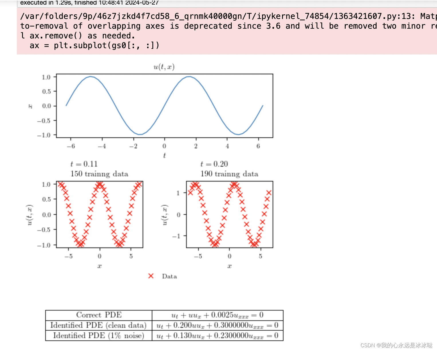
这里有一个知识点,关于这个gridspec函数
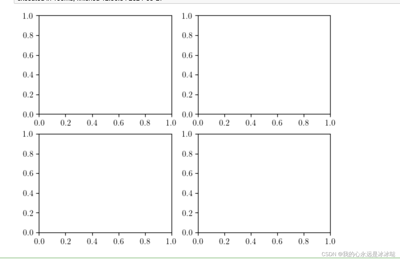
#导入模块
%matplotlib inline
import numpy as up
import matplotlib.pyplot as plt
import matplotlib.gridspec as gridspec

#创建画布实例
fig2 = plt.figure()

#创建 “区域规划图” 实例
#nrows=2,ncols=2 2行2列
spec2 = gridspec.GridSpec(nrows=2,ncols=2,figure=fig2)

#根据给定的 “区域规划图” ,创建对应的坐标系实例
ax1 = fig2.add_subplot(spec2[0,0])
ax2 = fig2.add_subplot(spec2[0,1])
ax3 = fig2.add_subplot(spec2[1,0])
ax4 = fig2.add_subplot(spec2[1,1])

#展示图表
plt.show()
example3(一张图)
# #!/usr/bin/env python3
# # -*- coding: utf-8 -*-
# """
# Created on Mon Oct  9 20:11:57 2017

# @author: mraissi
# """
import numpy as np
import matplotlib as mpl
#mpl.use('pgf')

def figsize(scale, nplots = 1):
    fig_width_pt = 390.0                          # Get this from LaTeX using \the\textwidth
    inches_per_pt = 1.0/72.27                       # Convert pt to inch
    golden_mean = (np.sqrt(5.0)-1.0)/2.0            # Aesthetic ratio (you could change this)
    fig_width = fig_width_pt*inches_per_pt*scale    # width in inches
    fig_height = nplots*fig_width*golden_mean              # height in inches
    fig_size = [fig_width,fig_height]
    return fig_size

pgf_with_latex = {                      # setup matplotlib to use latex for output
    "pgf.texsystem": "xelatex",        # change this if using xetex or lautex
    "text.usetex": True,                # use LaTeX to write all text
    "font.family": "serif",
    "font.serif": [],                   # blank entries should cause plots to inherit fonts from the document
    "font.sans-serif": [],
    "font.monospace": [],
    "axes.labelsize": 10,               # LaTeX default is 10pt font.
    "font.size": 10,
    "legend.fontsize": 8,               # Make the legend/label fonts a little smaller
    "xtick.labelsize": 8,
    "ytick.labelsize": 8,
    "figure.figsize": figsize(1.0),     # default fig size of 0.9 textwidth
    "pgf.preamble": "\n".join([
        r"\usepackage[utf8x]{inputenc}",    # use utf8 fonts becasue your computer can handle it :)
        r"\usepackage[T1]{fontenc}",        # plots will be generated using this preamble
        ]),
    }
mpl.rcParams.update(pgf_with_latex)

import matplotlib.pyplot as plt

# I make my own newfig and savefig functions
def newfig(width, nplots = 1):
    fig = plt.figure(figsize=figsize(width, nplots))
    ax = fig.add_subplot(111)
    return fig, ax

def savefig(filename, crop = True):
    if crop == True:
#        plt.savefig('{}.pgf'.format(filename), bbox_inches='tight', pad_inches=0)
        plt.savefig('{}.pdf'.format(filename), bbox_inches='tight', pad_inches=0)
        plt.savefig('{}.eps'.format(filename), bbox_inches='tight', pad_inches=0)
    else:
#        plt.savefig('{}.pgf'.format(filename))
        plt.savefig('{}.pdf'.format(filename))
        plt.savefig('{}.eps'.format(filename))


# import numpy as np
# import matplotlib.pyplot as plt
# #from plotting import newfig, savefig
# from mpl_toolkits.mplot3d import Axes3D
# import matplotlib.gridspec as gridspec
# from mpl_toolkits.axes_grid1 import make_axes_locatable

# fig, ax = newfig(1.0, 1.5)

# ax.axis('off')

# gs0 = gridspec.GridSpec(1, 2)
# gs0.update(top=1-0.06, bottom=1-1/3+0.05, left=0.15, right=0.85, wspace=0)
# ax = plt.subplot(gs0[:, :])

# # h = ax.imshow(Exact, interpolation='nearest', cmap='rainbow',
# #               extent=[t_star.min(),t_star.max(), lb[0], ub[0]],
# #               origin='lower', aspect='auto')
# # divider = make_axes_locatable(ax)
# # cax = divider.append_axes("right", size="5%", pad=0.05)
# # fig.colorbar(h, cax=cax)

# x = np.linspace(-2*np.pi, 2*np.pi)
# y = np.sin(x)
# ax.plot(x, y, '-', linewidth = 1.0)

# ax.set_xlabel('$t$')
# ax.set_ylabel('$x$')
# ax.set_title('$u(t,x)$', fontsize = 10)


# savefig('./AAAA')
import numpy as np
import matplotlib.pyplot as plt
#from plotting import newfig, savefig
from mpl_toolkits.mplot3d import Axes3D
import matplotlib.gridspec as gridspec
from mpl_toolkits.axes_grid1 import make_axes_locatable
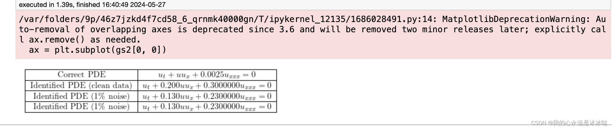
fig, ax = newfig(1.0, 0.5)
ax.axis('on')
gs2 = gridspec.GridSpec(1, 1)
gs2.update(top=0.8, bottom=0.5, left=0.15, right=0.85, wspace=0.0)
ax = plt.subplot(gs2[0, 0])
ax.axis('off')
s1 = r'$\begin{tabular}{ |c|c| } \hline Correct PDE & $u_t + u u_x + 0.0025 u_{xxx} = 0$ \\ \hline Identified PDE (clean data) & '
s2 = r'$u_t + %.3f u u_x + %.7f u_{xxx} = 0$ \\ \hline ' % (0.2, 0.3)
s3 = r'Identified PDE (1\% noise) & '
s4 = r'$u_t + %.3f u u_x + %.7f u_{xxx} = 0$ \\ \hline ' % (0.13, 0.23)
s5 = r'Identified PDE (1\% noise) & '
s6 = r'$u_t + %.3f u u_x + %.7f u_{xxx} = 0$ \\ \hline ' % (0.13, 0.23)
s100 = r'\end{tabular}$'
s = s1+s2+s3+s4+s5+s6+s100
ax.text(-0.1,0.2,s)
savefig('./BBBB')
example4(增加行列, 假如标题)
# #!/usr/bin/env python3
# # -*- coding: utf-8 -*-
# """
# Created on Mon Oct  9 20:11:57 2017

# @author: mraissi
# """
import numpy as np
import matplotlib as mpl
#mpl.use('pgf')

def figsize(scale, nplots = 1):
    fig_width_pt = 390.0                          # Get this from LaTeX using \the\textwidth
    inches_per_pt = 1.0/72.27                       # Convert pt to inch
    golden_mean = (np.sqrt(5.0)-1.0)/2.0            # Aesthetic ratio (you could change this)
    fig_width = fig_width_pt*inches_per_pt*scale    # width in inches
    fig_height = nplots*fig_width*golden_mean              # height in inches
    fig_size = [fig_width,fig_height]
    return fig_size

pgf_with_latex = {                      # setup matplotlib to use latex for output
    "pgf.texsystem": "xelatex",        # change this if using xetex or lautex
    "text.usetex": True,                # use LaTeX to write all text
    "font.family": "serif",
    "font.serif": [],                   # blank entries should cause plots to inherit fonts from the document
    "font.sans-serif": [],
    "font.monospace": [],
    "axes.labelsize": 10,               # LaTeX default is 10pt font.
    "font.size": 10,
    "legend.fontsize": 8,               # Make the legend/label fonts a little smaller
    "xtick.labelsize": 8,
    "ytick.labelsize": 8,
    "figure.figsize": figsize(1.0),     # default fig size of 0.9 textwidth
    "pgf.preamble": "\n".join([
        r"\usepackage[utf8x]{inputenc}",    # use utf8 fonts becasue your computer can handle it :)
        r"\usepackage[T1]{fontenc}",        # plots will be generated using this preamble
        ]),
    }
mpl.rcParams.update(pgf_with_latex)

import matplotlib.pyplot as plt

# I make my own newfig and savefig functions
def newfig(width, nplots = 1):
    fig = plt.figure(figsize=figsize(width, nplots))
    ax = fig.add_subplot(111)
    return fig, ax

def savefig(filename, crop = True):
    if crop == True:
#        plt.savefig('{}.pgf'.format(filename), bbox_inches='tight', pad_inches=0)
        plt.savefig('{}.pdf'.format(filename), bbox_inches='tight', pad_inches=0)
        plt.savefig('{}.eps'.format(filename), bbox_inches='tight', pad_inches=0)
    else:
#        plt.savefig('{}.pgf'.format(filename))
        plt.savefig('{}.pdf'.format(filename))
        plt.savefig('{}.eps'.format(filename))


# import numpy as np
# import matplotlib.pyplot as plt
# #from plotting import newfig, savefig
# from mpl_toolkits.mplot3d import Axes3D
# import matplotlib.gridspec as gridspec
# from mpl_toolkits.axes_grid1 import make_axes_locatable

# fig, ax = newfig(1.0, 1.5)

# ax.axis('off')

# gs0 = gridspec.GridSpec(1, 2)
# gs0.update(top=1-0.06, bottom=1-1/3+0.05, left=0.15, right=0.85, wspace=0)
# ax = plt.subplot(gs0[:, :])

# # h = ax.imshow(Exact, interpolation='nearest', cmap='rainbow',
# #               extent=[t_star.min(),t_star.max(), lb[0], ub[0]],
# #               origin='lower', aspect='auto')
# # divider = make_axes_locatable(ax)
# # cax = divider.append_axes("right", size="5%", pad=0.05)
# # fig.colorbar(h, cax=cax)

# x = np.linspace(-2*np.pi, 2*np.pi)
# y = np.sin(x)
# ax.plot(x, y, '-', linewidth = 1.0)

# ax.set_xlabel('$t$')
# ax.set_ylabel('$x$')
# ax.set_title('$u(t,x)$', fontsize = 10)


# savefig('./AAAA')
import numpy as np
import matplotlib.pyplot as plt
#from plotting import newfig, savefig
from mpl_toolkits.mplot3d import Axes3D
import matplotlib.gridspec as gridspec
from mpl_toolkits.axes_grid1 import make_axes_locatable
fig, ax = newfig(1.0, 0.5)
ax.axis('on')
gs2 = gridspec.GridSpec(1, 1)
gs2.update(top=0.8, bottom=0.5, left=0.15, right=0.85, wspace=0.0)
ax = plt.subplot(gs2[0, 0])
ax.axis('off')
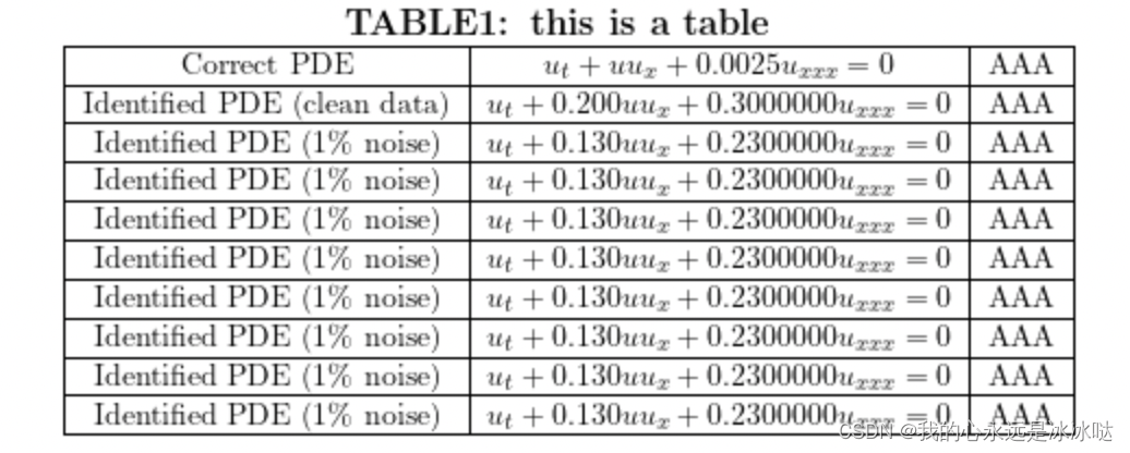
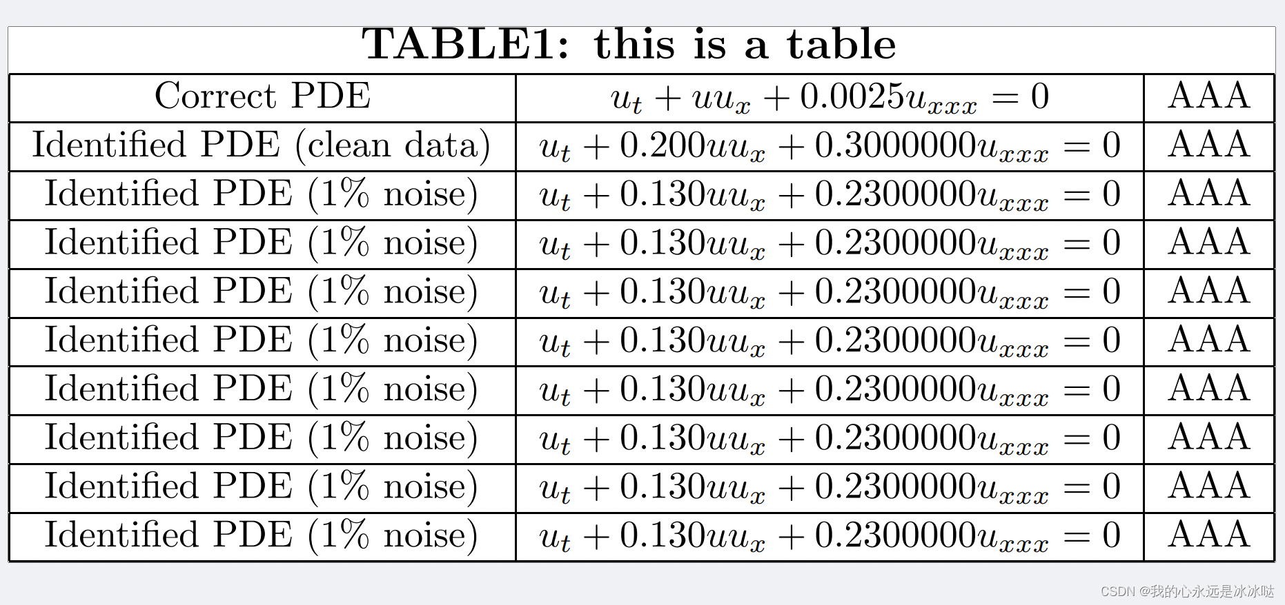
s1 = r'$\begin{tabular}{ |c|c|c| } \hline Correct PDE & $u_t + u u_x + 0.0025 u_{xxx} = 0$ &AAA \\ \hline Identified PDE (clean data) & '
s2 = r'$u_t + %.3f u u_x + %.7f u_{xxx} = 0$ & AAA\\ \hline ' % (0.2, 0.3)
s3 = r'Identified PDE (1\% noise) & '
s4 = r'$u_t + %.3f u u_x + %.7f u_{xxx} = 0$ & AAA \\ \hline ' % (0.13, 0.23)
s5 = r'Identified PDE (1\% noise) & '
s6 = r'$u_t + %.3f u u_x + %.7f u_{xxx} = 0$ & AAA \\ \hline ' % (0.13, 0.23)
s7 = r'Identified PDE (1\% noise) & '
s8 = r'$u_t + %.3f u u_x + %.7f u_{xxx} = 0$ & AAA \\ \hline ' % (0.13, 0.23)
s9 = r'Identified PDE (1\% noise) & '
s10 = r'$u_t + %.3f u u_x + %.7f u_{xxx} = 0$ & AAA \\ \hline ' % (0.13, 0.23)
s11 = r'Identified PDE (1\% noise) & '
s12 = r'$u_t + %.3f u u_x + %.7f u_{xxx} = 0$ & AAA \\ \hline ' % (0.13, 0.23)
s13 = r'Identified PDE (1\% noise) & '
s14 = r'$u_t + %.3f u u_x + %.7f u_{xxx} = 0$ & AAA \\ \hline ' % (0.13, 0.23)
s15 = r'Identified PDE (1\% noise) & '
s16 = r'$u_t + %.3f u u_x + %.7f u_{xxx} = 0$ & AAA \\ \hline ' % (0.13, 0.23)
s17 = r'Identified PDE (1\% noise) & '
s18 = r'$u_t + %.3f u u_x + %.7f u_{xxx} = 0$ & AAA \\ \hline ' % (0.13, 0.23)
s100 = r'\end{tabular}$'
s = s1+s2+s3+s4+s5+s6+s7+s8+s9+s10+s11+s12+s13+s14+s15+s16+s17+s18+s100
ax.text(-0.1,0.2,s)
ax.set_title(r"\textbf{TABLE1: this is a table}",y=2.0)
savefig('./BBBB')
example5(修改latex代码)
# #!/usr/bin/env python3
# # -*- coding: utf-8 -*-
# """
# Created on Mon Oct  9 20:11:57 2017

# @author: mraissi
# """
import numpy as np
import matplotlib as mpl
#mpl.use('pgf')

def figsize(scale, nplots = 1):
    fig_width_pt = 390.0                          # Get this from LaTeX using \the\textwidth
    inches_per_pt = 1.0/72.27                       # Convert pt to inch
    golden_mean = (np.sqrt(5.0)-1.0)/2.0            # Aesthetic ratio (you could change this)
    fig_width = fig_width_pt*inches_per_pt*scale    # width in inches
    fig_height = nplots*fig_width*golden_mean              # height in inches
    fig_size = [fig_width,fig_height]
    return fig_size

pgf_with_latex = {                      # setup matplotlib to use latex for output
    "pgf.texsystem": "xelatex",        # change this if using xetex or lautex
    "text.usetex": True,                # use LaTeX to write all text
    "font.family": "serif",
    "font.serif": [],                   # blank entries should cause plots to inherit fonts from the document
    "font.sans-serif": [],
    "font.monospace": [],
    "axes.labelsize": 10,               # LaTeX default is 10pt font.
    "font.size": 10,
    "legend.fontsize": 8,               # Make the legend/label fonts a little smaller
    "xtick.labelsize": 8,
    "ytick.labelsize": 8,
    "figure.figsize": figsize(1.0),     # default fig size of 0.9 textwidth
    "pgf.preamble": "\n".join([
        r"\usepackage[utf8x]{inputenc}",    # use utf8 fonts becasue your computer can handle it :)
        r"\usepackage[T1]{fontenc}",        # plots will be generated using this preamble
        ]),
    }
mpl.rcParams.update(pgf_with_latex)

import matplotlib.pyplot as plt

# I make my own newfig and savefig functions
def newfig(width, nplots = 1):
    fig = plt.figure(figsize=figsize(width, nplots))
    ax = fig.add_subplot(111)
    return fig, ax

def savefig(filename, crop = True):
    if crop == True:
#        plt.savefig('{}.pgf'.format(filename), bbox_inches='tight', pad_inches=0)
        plt.savefig('{}.pdf'.format(filename), bbox_inches='tight', pad_inches=0)
        plt.savefig('{}.eps'.format(filename), bbox_inches='tight', pad_inches=0)
    else:
#        plt.savefig('{}.pgf'.format(filename))
        plt.savefig('{}.pdf'.format(filename))
        plt.savefig('{}.eps'.format(filename))


# import numpy as np
# import matplotlib.pyplot as plt
# #from plotting import newfig, savefig
# from mpl_toolkits.mplot3d import Axes3D
# import matplotlib.gridspec as gridspec
# from mpl_toolkits.axes_grid1 import make_axes_locatable

# fig, ax = newfig(1.0, 1.5)

# ax.axis('off')

# gs0 = gridspec.GridSpec(1, 2)
# gs0.update(top=1-0.06, bottom=1-1/3+0.05, left=0.15, right=0.85, wspace=0)
# ax = plt.subplot(gs0[:, :])

# # h = ax.imshow(Exact, interpolation='nearest', cmap='rainbow',
# #               extent=[t_star.min(),t_star.max(), lb[0], ub[0]],
# #               origin='lower', aspect='auto')
# # divider = make_axes_locatable(ax)
# # cax = divider.append_axes("right", size="5%", pad=0.05)
# # fig.colorbar(h, cax=cax)

# x = np.linspace(-2*np.pi, 2*np.pi)
# y = np.sin(x)
# ax.plot(x, y, '-', linewidth = 1.0)

# ax.set_xlabel('$t$')
# ax.set_ylabel('$x$')
# ax.set_title('$u(t,x)$', fontsize = 10)


# savefig('./AAAA')
import numpy as np
import matplotlib.pyplot as plt
#from plotting import newfig, savefig
from mpl_toolkits.mplot3d import Axes3D
import matplotlib.gridspec as gridspec
from mpl_toolkits.axes_grid1 import make_axes_locatable
fig, ax = newfig(1.0, 0.52)
ax.axis('on')
gs2 = gridspec.GridSpec(1, 1)
#gs2.update(top=0.8, bottom=0.5, left=0.15, right=0.85, wspace=0.0)
gs2.update(top=1-2/3-0.05, bottom=0, left=0.15, right=0.85, wspace=0.0)
ax = plt.subplot(gs2[0, 0])
ax.axis('off')
## 可以调整这个结果了,嘿嘿,还是很好的哈。
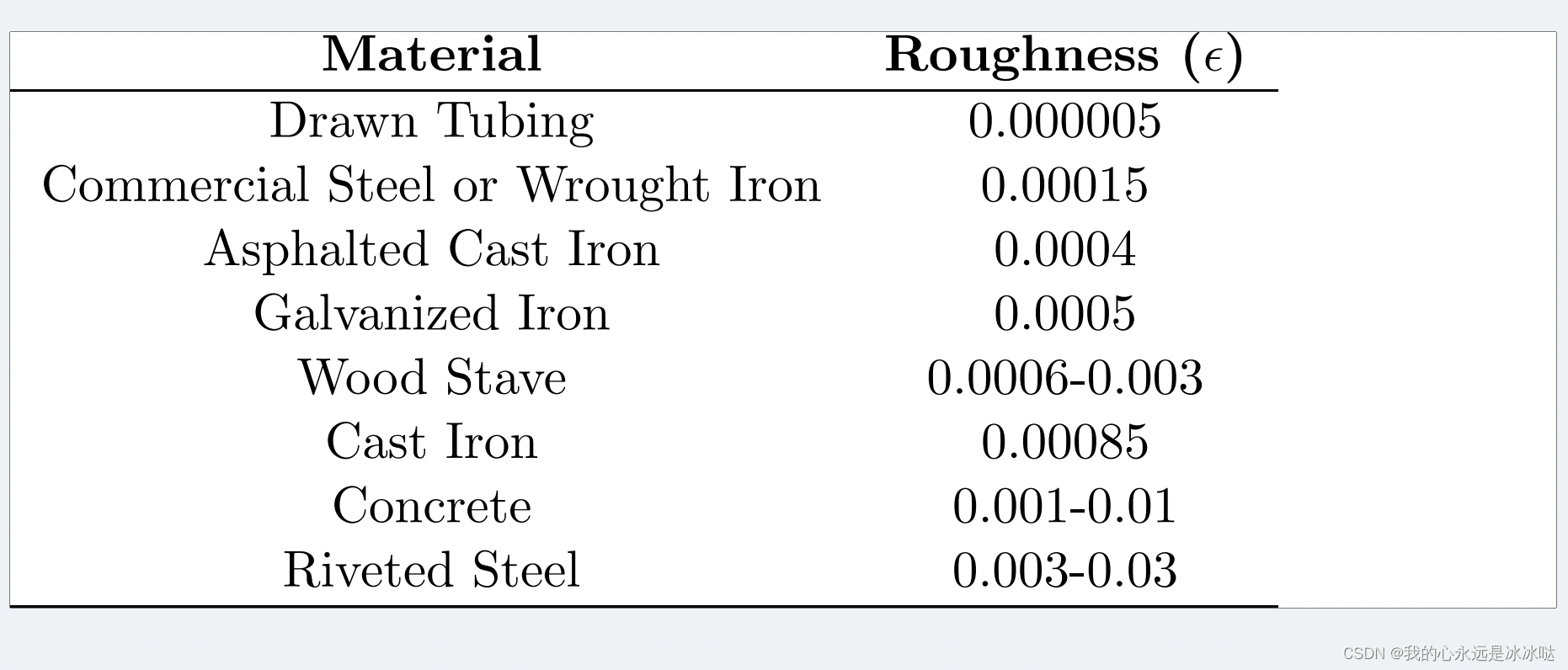
table = (r"\begin{tabular}{cc}"
r"\bf{Material} & \bf{Roughness ($\epsilon$)} \\"
r"\hline "
r"Drawn Tubing & 0.000005 \\"
r"Commercial Steel or Wrought Iron & 0.00015 \\"
r"Asphalted Cast Iron & 0.0004 \\"
r"Galvanized Iron & 0.0005 \\"
r"Wood Stave & 0.0006-0.003 \\"
r"Cast Iron & 0.00085 \\"
r"Concrete & 0.001-0.01 \\"
r"Riveted Steel & 0.003-0.03 \\"
r"\hline "
r"\end{tabular}")
ax.text(-0.1,0.2,table)
#ax.set_title(r"\textbf{TABLE1: this is a table}",y=2.0)
savefig('./CCCC')
结果如下


 812
812

 被折叠的 条评论
为什么被折叠?
被折叠的 条评论
为什么被折叠?
 到【灌水乐园】发言


