matplotlib常用方法

---

1.基础

# Basic
plt.figure(num=1, figsize=(8,5))
x = np.linspace(-np.pi,np.pi,20)
y = np.sin(x)
plt.plot(x,y,color='red',linewidth=1.0,linestyle='--',marker='*',markerfacecolor='blue',markersize=10)
plt.show()

# multiple lines
plt.figure(num=2, figsize=(8,5))
x = np.arange(10)
y = np.arange(0,5,0.5)
plt.plot(x,y,'r--',
		x,y**2,'bs',
 		x,y**3,'g^')
plt.show()

# return object
plt.figure(num=3, figsize=(8,5))
x = np.linspace(-np.pi,np.pi,20)
y1 = np.sin(x)
y2 = np.cos(x)
y3 = np.tan(x)
line1,line2,line3 = plt.plot(x,y1,x,y2,x,y3)
line1.set(color='b',linewidth=4.0,antialiased=False)
line2.set_antialiased(False)
line2.set_linewidth(4.0)
line2.set_color('red')
plt.setp(line3,color='k',linewidth=4.0)
plt.show()

2.图例

# Legend
# method 1
x = np.linspace(-3,3,10)
y1 = 2*x+1
y2 = x**2
l1,=plt.plot(x,y1,label='line1')
l2,=plt.plot(x,y2,label='line2')
plt.legend()
# method 2
l1,=plt.plot(x,y1)
l2,=plt.plot(x,y2)
fontdict = {'family' : 'Times New Roman',
		'weight' : 'normal',
		'size' : 13,
}
legend = plt.legend(handles=[l1,l2],labels=['line1','line2'], prop=fontdict)

3.坐标设置

# Axis setting
# label
plt.xlabel("Im x")
plt.ylabel("Im y")
# limit
plt.xlim((-3,3))
plt.ylim((-5,5))
# ticks
plt.xticks(np.linspace(-3,3,9))
plt.yticks([-5,-2,0,2,5], ['very low','low','normal','high','very high'])
# gca(): get current axis
ax = plt.gca()
ax.spines['right'].set_color('none')
ax.spines['top'].set_color('none')
# coordinate display position
ax.xaxis.set_ticks_position('top')
ax.yaxis.set_ticks_position('right')
# set axis position
ax.spines['bottom'].set_position(('data',0))	#data axes
ax.spines['left'].set_position(('data',0))
# tick labels
for label in ax.get_xticklabels() + ax.get_yticklabels():
	label.set_fontsize(12)
	label.set_bbox(dict(facecolor='red',edgecolor='None',alpha=0.7))

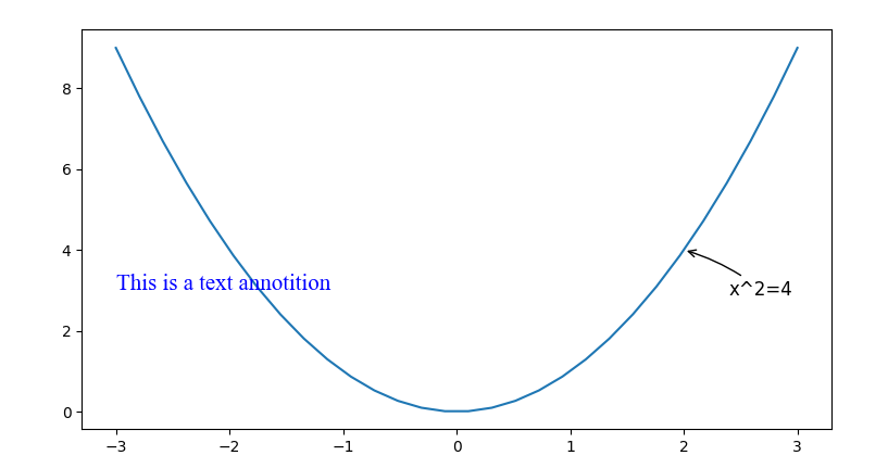
4.注释和文本标注

# Annotation
x = np.linspace(-3,3,30)
y = x**2
x0 = 2
y0 = x0**2
plt.plot(x,y)
# annotate
plt.annotate('x^2=%d'%y0,xy=(x0,y0),xycoords='data',xytext=(+30,-30),textcoords='offset points',
			fontsize=12,arrowprops=dict(arrowstyle='->',connectionstyle='arc3,rad=.1'))

# text
fontdict = {'family' : 'Times New Roman',
		'weight' : 'normal',
		'size' : 15,
		'color' : 'blue'
}
plt.text(-3,3,'This is a text annotition',fontdict=fontdict)
plt.show()

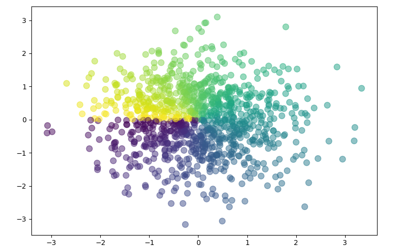
5.散点图

# Scatter
X = np.random.normal(0,1,1024)
Y = np.random.normal(0,1,1024)
colors= np.arctan2(Y,X)
plt.scatter(X,Y,s=75,c=colors,alpha=0.5)
plt.show()

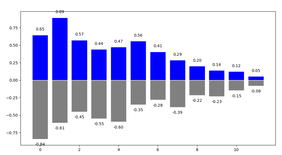
6.条形图

# Bar
X = np.arange(12)
Y1 = (1-X/float(n))*np.random.uniform(0.5,1.0,n)
Y2 = (1-X/float(n))*np.random.uniform(0.5,1.0,n)
plt.bar(X,+Y1,facecolor='blue',edgecolor='white')
plt.bar(X,-Y2,facecolor='grey',edgecolor='white')
# label
for x,y in zip(X,Y1):
	plt.text(x,y+0.05,'%.2f'%y,ha='center',va='bottom')
for x,y in zip(X,Y2):
	plt.text(x,-y-0.05,'-%.2f'%y,ha='center',va='top')
plt.show()

7.等高线图

# Contours
# backstepping function
def f(x,y):
	return x**2 + y**2
# meshgrid
n= 256
x = np.linspace(-3,3,n)
y = np.linspace(-3,3,n)
X,Y = np.meshgrid(x,y)
# use plt.contourf to filling contours
plt.contourf(X,Y,f(X,Y),8,alpha=0.75,cmap=plt.cm.coolwarm)  #cool
# use plt.contour to add contour lines
C = plt.contour(X,Y,f(X,Y),10,colors='black',linewidth=0.5)
# adding label
plt.clabel(C,inline=True,fontsize=10)
plt.show()

8.3D

from mpl_toolkits.mplot3d import Axes3D

#3D
fig = plt.figure(0)
ax = Axes3D(fig)
X = np.linspace(-4,4,20)
Y = np.linspace(-4,4,20)
X,Y = np.meshgrid(X,Y)
R = np.sqrt(X**2 +Y**2)
Z = np.sin(R)
ax.set_xlim(-4,4)
ax.set_ylim(-4,4)
ax.set_zlim(-2,2)
# surface
ax.plot_surface(X,Y,Z,rstride=1,cstride=1,cmap=plt.get_cmap('rainbow'))
# contourf
ax.contourf(X,Y,Z,zdir='z',offset=-2,cmap='rainbow')
plt.show()

9.subplot

#Subplot
#subplot
plt.figure()
plt.subplot(221)
plt.plot([0,1],[0,1])
plt.subplot(222)
plt.plot([0,1],[0,1])
plt.subplot(233)
plt.plot([0,1],[0,1])
#subplot2grid
fg1 = plt.subplot2grid((3,3),(0,0),colspan=3,rowspan=1)
fg2 = plt.subplot2grid((3,3),(1,0),colspan=2,rowspan=1)
fg3 = plt.subplot2grid((3,3),(1,2),colspan=1,rowspan=2)
gg4 = plt.subplot2grid((3,3),(2,0))
#gridspec
gs = gridspec.GridSpec(3,3)
fg1 = plt.subplot(gs[0,:])
fg2 = plt.subplot(gs[1,0:1])
fg3 = plt.subplot(gs[1:,1:])
plt.show()

10.图中图

#plot in plot
fig = plt.figure()
x = np.arange(5)
y = np.arange(5)
left,bottom,width,height = 0.1,0.1,0.8,0.8
ax1 = fig.add_axes([left,bottom,width,height])
ax1.plot(x,y)
left,bottom,width,height = 0.2,0.5,0.3,0.3
ax2 = fig.add_axes([left,bottom,width,height])
ax2.plot(x,y)
plt.show()

11.动画

#animation
fig, ax = plt.subplots()
x = np.arange(0,2*np.pi,0.01)
line,=ax.plot(x,np.sin(x))
def animate(i):
	line.set_ydata(np.sin(x+i/100))
	return line
def init():
	line.set_ydata(np.sin(x))
	return line
ani = animation.FuncAnimation(fig=fig, func=animate, frames=100, 
							init_func=init, interval=20, blit=False)
plt.show()