【深度学习——猴痘病识别】

• 🍨 本文为🔗365天深度学习训练营 中的学习记录博客
• 🍖 原作者：K同学啊 | 接辅导、项目定制
• 🚀 文章来源：K同学的学习圈子

一、前期准备工作

1、设置GPU

from tensorflow import keras
from tensorflow.keras import layers,models
import os,PIL,pathlib

import matplotlib.pyplot as plt
import tensorflow as tf

gpus=tf.config.list_physical_devices("GPU")
if gpus:
    gpus0=gpus[0]
    tf.config.experimental.set_memory_growth(gpus0,True)
    tf.config.set_visible_devices([gpus0],"GPU")
gpus

2、导入数据

data_dir="D:\桌面\深度学习数据\第4周"
data_dir=pathlib.Path(data_dir)

3、查看数据

image_count = len(list(data_dir.glob('*/*.jpg')))
print("图片总数为：",image_count)

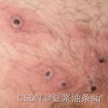
查看病毒数据集的第一张数据图片

Monkeypox = list(data_dir.glob('Monkeypox/*.jpg'))
PIL.Image.open(str(Monkeypox[0]))

二、数据预处理

1、加载数据

使用image_dataset_from_directory方法将磁盘中的数据加载到tf.data.Dataset中
测试集与验证集的关系：
1.验证集并没有参与训练过程梯度下降过程的，狭义上来讲是没有参与模型的参数训练更新的。
2.但是广义上来讲，验证集存在的意义确实参与了一个“人工调参”的过程，我们根据每一个epoch训练之后模型在valid data上的表现来决定是否需要训练进行early stop，或者根据这个过程模型的性能变化来调整模型的超参数，如学习率，batch_size等等。
3.因此也可以认为，验证集也参与了训练，但是并没有使得模型去overfit验证集

batch_size = 32
img_height = 224
img_width = 224

train_ds = tf.keras.preprocessing.image_dataset_from_directory(
    data_dir,
    validation_split=0.2,
    subset="training",
    seed=123,
    image_size=(img_height, img_width),
    batch_size=batch_size)

val_ds = tf.keras.preprocessing.image_dataset_from_directory(
    data_dir,
    validation_split=0.2,
    subset="validation",
    seed=123,
    image_size=(img_height, img_width),
    batch_size=batch_size)

通过class_names输出数据集的标签。标签将按字母顺序对应于目录名称

class_names = train_ds.class_names
print(class_names)

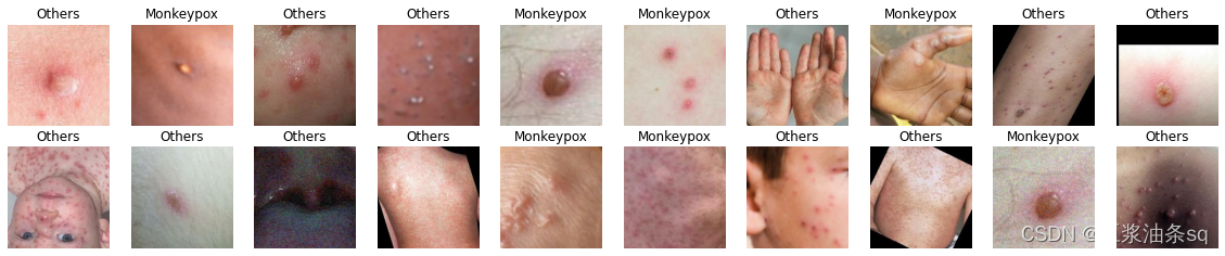
2、可视化数据

plt.figure(figsize=(20, 10))

for images, labels in train_ds.take(1):
    for i in range(20):
        ax = plt.subplot(5, 10, i + 1)

        plt.imshow(images[i].numpy().astype("uint8"))
        plt.title(class_names[labels[i]])
        
        plt.axis("off")

3、再次检查数据

for image_batch, labels_batch in train_ds:
    print(image_batch.shape)
    print(labels_batch.shape)
    break

• Image_batch是形状的张量（32,180,180,3）。这是一批形状180x180x3的32张图片（最后一维指的是彩色通道RGB）。
• Label_batch是形状（32，）的张量，这些标签对应32张图片

4、配置数据集

• huffle() ：打乱数据
• prefetch() ：预取数据，加速运行

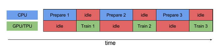
prefetch()功能详细介绍：CPU 正在准备数据时，加速器处于空闲状态。

相反，当加速器正在训练模型时，CPU 处于空闲状态。

因此，训练所用的时间是 CPU 预处理时间和加速器训练时间的总和。

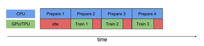
prefetch()将训练步骤的预处理和模型执行过程重叠到一起。当加速器正在执行第 N 个训练步时，CPU 正在准备第 N+1 步的数据。这样做不仅可以最大限度地缩短训练的单步用时（而不是总用时），而且可以缩短提取和转换数据所需的时间。

如果不使用prefetch()，CPU 和 GPU/TPU 在大部分时间都处于空闲状态：

使用prefetch()可显著减少空闲时间：

• cache() ：将数据集缓存到内存当中，加速运行

AUTOTUNE = tf.data.AUTOTUNE

train_ds = train_ds.cache().shuffle(1000).prefetch(buffer_size=AUTOTUNE)
val_ds = val_ds.cache().prefetch(buffer_size=AUTOTUNE)

三、构建CNN网络

卷积神经网络（CNN）的输入是张量 (Tensor) 形式的 (image_height, image_width, color_channels)，包含了图像高度、宽度及颜色信息。
不需要输入batch size。
color_channels 为 (R,G,B) 分别对应 RGB 的三个颜色通道（color channel）。
在此示例中，CNN 输入的形状是 (224, 224, 4)即彩色图像。需要在声明第一层时将形状赋值给参数input_shape。
网络结构构图：

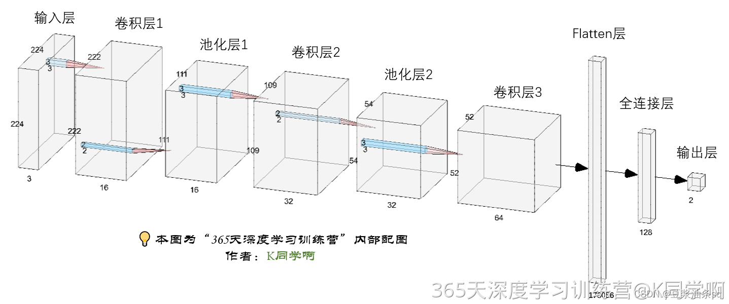
num_classes = 2

model = models.Sequential([
    layers.experimental.preprocessing.Rescaling(1./255, input_shape=(img_height, img_width, 3)),
    
    layers.Conv2D(16, (3, 3), activation='relu', input_shape=(img_height, img_width, 3)), # 卷积层1，卷积核3*3  
    layers.AveragePooling2D((2, 2)),               # 池化层1，2*2采样
    layers.Conv2D(32, (3, 3), activation='relu'),  # 卷积层2，卷积核3*3
    layers.AveragePooling2D((2, 2)),               # 池化层2，2*2采样
    layers.Dropout(0.3),  
    layers.Conv2D(64, (3, 3), activation='relu'),  # 卷积层3，卷积核3*3
    layers.Dropout(0.3),  
    
    layers.Flatten(),                       # Flatten层，连接卷积层与全连接层
    layers.Dense(128, activation='relu'),   # 全连接层，特征进一步提取
    layers.Dense(num_classes)               # 输出层，输出预期结果
])

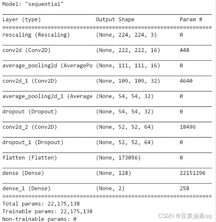
model.summary()  # 打印网络结构

四、编译

• 损失函数（loss）：用于衡量模型在训练期间的准确率。
• 优化器（optimizer）：决定模型如何根据其看到的数据和自身的损失函数进行更新。
• 指标（metrics）：用于监控训练和测试步骤。以下示例使用了准确率，即被正确分类的图像的比率。

# 设置优化器
opt = tf.keras.optimizers.Adam(learning_rate=1e-4)
model.compile(optimizer=opt,loss=tf.keras.losses.SparseCategoricalCrossentropy(from_logits=True),metrics=['accuracy'])

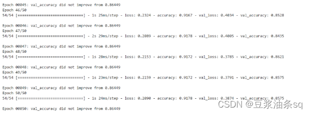
五、训练模型

from tensorflow.keras.callbacks import ModelCheckpoint

epochs = 50

checkpointer = ModelCheckpoint('best_model.h5',
                                monitor='val_accuracy',
                                verbose=1,
                                save_best_only=True,
                                save_weights_only=True)

history = model.fit(train_ds,
                    validation_data=val_ds,
                    epochs=epochs,
                    callbacks=[checkpointer])

六、模型评估

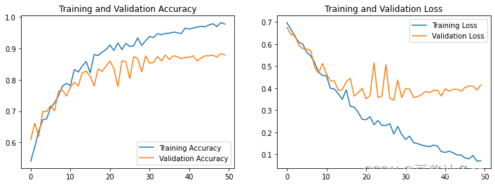
1、Loss与Accuracy图

acc = history.history['accuracy']
val_acc = history.history['val_accuracy']

loss = history.history['loss']
val_loss = history.history['val_loss']

epochs_range = range(epochs)

plt.figure(figsize=(12, 4))
plt.subplot(1, 2, 1)
plt.plot(epochs_range, acc, label='Training Accuracy')
plt.plot(epochs_range, val_acc, label='Validation Accuracy')
plt.legend(loc='lower right')
plt.title('Training and Validation Accuracy')

plt.subplot(1, 2, 2)
plt.plot(epochs_range, loss, label='Training Loss')
plt.plot(epochs_range, val_loss, label='Validation Loss')
plt.legend(loc='upper right')
plt.title('Training and Validation Loss')
plt.show()

2、指定图片进行预测

# 加载效果最好的模型权重
model.load_weights('best_model.h5')

from PIL import Image
import numpy as np

img = Image.open("MonkeyData/Monkeypox/M06_01_04.jpg")  #这里选择需要预测的图片
# img = Image.open("MonkeyData/Others/NM15_02_11.jpg")  #这里选择需要预测的图片
image = tf.image.resize(img, [img_height, img_width])

img_array = tf.expand_dims(image, 0) 

predictions = model.predict(img_array) # 这里选用已经训练好的模型
print("预测结果为：",class_names[np.argmax(predictions)])

预测结果为：Others