机器学习之惩罚回归—基于python实现（附完整代码）

      大家好，我是带我去滑雪！

      本期为大家介绍惩罚回归，分别从以下几个方面着手：为什么会有惩罚回归？什么是惩罚回归？常见的惩罚回归有哪些？惩罚回归的python代码如何实现？我相信解决好这些问题，就已经基本能够掌握惩罚回归的很多知识。话不多说，开始学习！

目录

       1、为什么会有惩罚回归？

2、什么是惩罚回归？

3、常见的惩罚回归有哪些？

4、惩罚回归的python代码实现

（1）由于此csv文件以分号 “；”分割，故使用命令“pd.read_table('student-mat.csv',sep=';')”载入数据，并考察此数据框的形状与前5个观测值

（2）从数据集中去掉变量G1和G2，因为这是同一学期的前两阶段成绩，且与G3高度相关

（4）使用函数pd.get_dummies()将数据矩阵中的分类变量都变为虚拟变量

（5）将所有特征变量标准化

（6）考虑惩罚参数​alpha的网格np.logspace(-3，6，100)，画出岭回归的系数路径

 （7）通过10折交叉验证（使用random-state=1），选择最优惩罚参数​编辑，进行岭回归，以数据框的形式展示最优岭回归的系数，并画出交叉验证图

（8）设定参数“eps=le-4”，使用lasso_path()函数，画出lasso回归的系数路径

（9）通过10折交叉验证（使用random-state=1），在网格np.logspace(-3，1，100)上选择最优惩罚参数​编辑，进行Lasso回归，并以数据框的形式展示最优Lasso回归的系数

（10）考虑惩罚参数​alpha的网格np.logspace(-3，1，100)与调节参数11_ratio的网格[0.001，0.01，0.1，0.5，1]，并通过10折交叉验证（使用random-state=1）,选择最优参数​编辑与11_ratio，进行弹性网回归，汇报样本内的拟合优度，并以数据框的形式展示最优弹性网回归的系数

（11）使用random-state=0，随机预留100个观测值作为测试集，进行最优的弹性网回归，分别计算训练集与测试集的拟合优度

---

1、为什么会有惩罚回归？

       当前，我们所要处理的数据通常表现为高维数据，即特征变量的维度远远大于样本容量。例如，当进行一项医学研究时，需要研究哪些基因会引起病人肥胖，由于成本限制仅收集到200位病人的信息，其中每位病人均有20000条基因，可以发现样本容量为200，但特征变量个数却高达20000。这样的例子，在当前这个大数据时代，是常见的。如此多变量虽然可以提高更多的信息，但同时也对传统线性回归估计带来了挑战。在高维数据中，特征变量个数过多，特征变量之间势必会存在多重共线性，普通最小二乘法（OLS）不存在唯一解，无法利用OLS进行高维回归。如果使用传统的OLS回归，会出现模型过度拟合，模型外推预测的效果欠佳（ps：过拟合指模型在训练集中表现良好，但在测试集中表现不好）。因此，为了解决过拟合问题，提出了惩罚回归模型。

2、什么是惩罚回归？

        惩罚回归是指即在目标函数中增加一个惩罚项，使模型系数个数收缩，降低模型的复杂度。

3、常见的惩罚回归有哪些？

        常见的惩罚回归有岭回归（ridge regression）、Lasso回归和弹性网络回归（Elastic-net regression）。岭回归也叫线性回归的 L2 正则化，它将系数值缩小到接近零，但不删除任何变量。岭回归可以提高预测精准度，但在模型的解释上会更加的复杂化。LASSO 回归也叫线性回归的 L1 正则化，该方法最突出的优势在于通过对所有变量系数进行回归惩罚，使得相对不重要的独立变量系数变为 0，从而被排除在建模之外。因此，它在拟合模型的同时进行特征选择。弹性网络是同时使用了系数向量的L1 范数和L2 范数的线性回归模型，使得可以学习得到类似于Lasso的一个稀疏模型，同时还保留了 Ridge 的正则化属性，结合了二者的优点，尤其适用于有多个特征彼此相关的场合。

4、惩罚回归的python代码实现

       使用UCI Machine Learning Repository 的葡萄牙高中数学成绩数据student-mat.csv，进行惩罚回归，该数据集中G3为期末成绩，而school、sex、address、famsize、Pstatus等共计32个变量为特征变量。期望完成如下任务：

（1）由于此csv文件以分号 “；”分割，故使用命令“pd.read_table('student-mat.csv',sep=';')”载入数据，并考察此数据框的形状与前5个观测值；

（2）从数据集中去掉变量G1和G2，因为这是同一学期的前两阶段成绩，且与G3高度相关；

（3）画出响应变量G3的直方图；

（4）使用函数pd.get_dummies()将数据矩阵中的分类变量都变为虚拟变量；

（5）将所有特征变量标准化；

（6）考虑惩罚参数的网格np.logspace(-3，6，100)，画出岭回归的系数路径；

（7）通过10折交叉验证（使用random-state=1），选择最优惩罚参数，进行岭回归，并以数据框的形式展示最优岭回归的系数；

（8）设定参数“eps=le-4”，使用lasso_path()函数，画出lasso回归的系数路径；

（9）通过10折交叉验证（使用random-state=1），在网格np.logspace(-3，1，100)上选择最优惩罚参数，进行Lasso回归，并以数据框的形式展示最优Lasso回归的系数；

（10）考虑惩罚参数的网格np.logspace(-3，1，100)与调节参数11_ratio的网格[0.001，0.01，0.1，0.5，1]，并通过10折交叉验证（使用random-state=1）,选择最优参数与11_ratio，进行弹性网回归，汇报样本内的拟合优度，并以数据框的形式展示最优弹性网回归的系数；

（11）使用random-state=0，随机预留100个观测值作为测试集，进行最优的弹性网回归，分别计算训练集与测试集的拟合优度。

         首先导入本案例所需的所有模块：

import numpy as np
import pandas as pd
import matplotlib.pyplot as plt
from sklearn.model_selection import train_test_split
from sklearn.model_selection import KFold
from sklearn.model_selection import cross_val_score
from sklearn.preprocessing import StandardScaler
 
from sklearn.linear_model import Ridge
from sklearn.linear_model import RidgeCV
from sklearn.linear_model import Lasso
from sklearn.linear_model import lasso_path
from sklearn.linear_model import LassoCV
from sklearn.linear_model import ElasticNet
from sklearn.linear_model import ElasticNetCV
from sklearn.linear_model import enet_path

（1）由于此csv文件以分号 “；”分割，故使用命令“pd.read_table('student-mat.csv',sep=';')”载入数据，并考察此数据框的形状与前5个观测值

student_mat=pd.read_table(r'E:\工作\硕士\博客\博客25-惩罚回归\student-mat.csv',sep=';')
student_mat

输出结果：

	school	sex	age	address	famsize	Pstatus	Medu	Fedu	Mjob	Fjob	...	famrel	freetime	goout	Dalc	Walc	health	absences	G1	G2	G3
0	GP	F	18	U	GT3	A	4	4	at_home	teacher	...	4	3	4	1	1	3	6	5	6	6
1	GP	F	17	U	GT3	T	1	1	at_home	other	...	5	3	3	1	1	3	4	5	5	6
2	GP	F	15	U	LE3	T	1	1	at_home	other	...	4	3	2	2	3	3	10	7	8	10
3	GP	F	15	U	GT3	T	4	2	health	services	...	3	2	2	1	1	5	2	15	14	15
4	GP	F	16	U	GT3	T	3	3	other	other	...	4	3	2	1	2	5	4	6	10	10
...	...	...	...	...	...	...	...	...	...	...	...	...	...	...	...	...	...	...	...	...	...
390	MS	M	20	U	LE3	A	2	2	services	services	...	5	5	4	4	5	4	11	9	9	9
391	MS	M	17	U	LE3	T	3	1	services	services	...	2	4	5	3	4	2	3	14	16	16
392	MS	M	21	R	GT3	T	1	1	other	other	...	5	5	3	3	3	3	3	10	8	7
393	MS	M	18	R	LE3	T	3	2	services	other	...	4	4	1	3	4	5	0	11	12	10
394	MS	M	19	U	LE3	T	1	1	other	at_home	...	3	2	3	3	3	5	5	8	9	9

395 rows × 33 columns

student_mat.shape#展示数据框形状

输出结果：

(395, 33)

student_mat.head()#考察数据框前5个观测值

输出结果：

	school	sex	age	address	famsize	Pstatus	Medu	Fedu	Mjob	Fjob	...	famrel	freetime	goout	Dalc	Walc	health	absences	G1	G2	G3
0	GP	F	18	U	GT3	A	4	4	at_home	teacher	...	4	3	4	1	1	3	6	5	6	6
1	GP	F	17	U	GT3	T	1	1	at_home	other	...	5	3	3	1	1	3	4	5	5	6
2	GP	F	15	U	LE3	T	1	1	at_home	other	...	4	3	2	2	3	3	10	7	8	10
3	GP	F	15	U	GT3	T	4	2	health	services	...	3	2	2	1	1	5	2	15	14	15
4	GP	F	16	U	GT3	T	3	3	other	other	...	4	3	2	1	2	5	4	6	10	10

5 rows × 33 columns

​

（2）从数据集中去掉变量G1和G2，因为这是同一学期的前两阶段成绩，且与G3高度相关

student=student_mat.drop(['G1', 'G2'], axis=1)
student

输出结果：

	school	sex	age	address	famsize	Pstatus	Medu	Fedu	Mjob	Fjob	...	internet	romantic	famrel	freetime	goout	Dalc	Walc	health	absences	G3
0	GP	F	18	U	GT3	A	4	4	at_home	teacher	...	no	no	4	3	4	1	1	3	6	6
1	GP	F	17	U	GT3	T	1	1	at_home	other	...	yes	no	5	3	3	1	1	3	4	6
2	GP	F	15	U	LE3	T	1	1	at_home	other	...	yes	no	4	3	2	2	3	3	10	10
3	GP	F	15	U	GT3	T	4	2	health	services	...	yes	yes	3	2	2	1	1	5	2	15
4	GP	F	16	U	GT3	T	3	3	other	other	...	no	no	4	3	2	1	2	5	4	10
...	...	...	...	...	...	...	...	...	...	...	...	...	...	...	...	...	...	...	...	...	...
390	MS	M	20	U	LE3	A	2	2	services	services	...	no	no	5	5	4	4	5	4	11	9
391	MS	M	17	U	LE3	T	3	1	services	services	...	yes	no	2	4	5	3	4	2	3	16
392	MS	M	21	R	GT3	T	1	1	other	other	...	no	no	5	5	3	3	3	3	3	7
393	MS	M	18	R	LE3	T	3	2	services	other	...	yes	no	4	4	1	3	4	5	0	10
394	MS	M	19	U	LE3	T	1	1	other	at_home	...	yes	no	3	2	3	3	3	5	5	9

395 rows × 31 columns

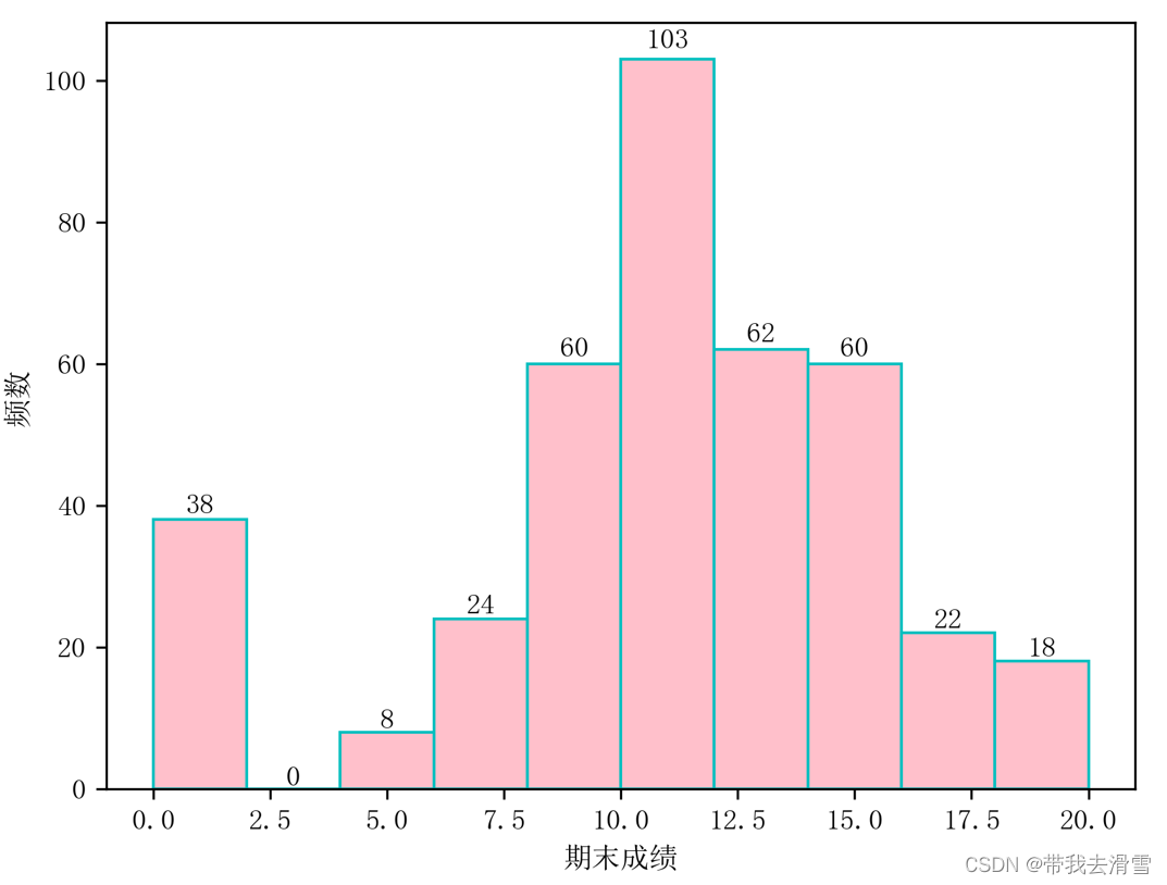
（3）画出响应变量G3的直方图；

plt.rcParams['font.sans-serif'] = ['SimSun'] #'画图使中文正常显示为宋体
n, bins, patches = plt.hist(student.G3,color='pink',edgecolor='c', bins=10)

for i in range(len(n)):
    plt.text(bins[i]+(bins[1]-bins[0])/2, n[i]*1.01, int(n[i]), ha='center', va= 'bottom')
plt.xlabel("期末成绩")
plt.ylabel(" 频数")
plt.savefig("squares7.png",
            bbox_inches ="tight",
            pad_inches = 0.5,
            transparent = True,
            facecolor ="w",
            edgecolor ='w',
            dpi=300,
            orientation ='landscape')

输出结果：

（4）使用函数pd.get_dummies()将数据矩阵中的分类变量都变为虚拟变量

dd=pd.get_dummies(student)
dd

输出结果：

	age	Medu	Fedu	traveltime	studytime	failures	famrel	freetime	goout	Dalc	...	activities_no	activities_yes	nursery_no	nursery_yes	higher_no	higher_yes	internet_no	internet_yes	romantic_no	romantic_yes
0	18	4	4	2	2	0	4	3	4	1	...	1	0	0	1	0	1	1	0	1	0
1	17	1	1	1	2	0	5	3	3	1	...	1	0	1	0	0	1	0	1	1	0
2	15	1	1	1	2	3	4	3	2	2	...	1	0	0	1	0	1	0	1	1	0
3	15	4	2	1	3	0	3	2	2	1	...	0	1	0	1	0	1	0	1	0	1
4	16	3	3	1	2	0	4	3	2	1	...	1	0	0	1	0	1	1	0	1	0
...	...	...	...	...	...	...	...	...	...	...	...	...	...	...	...	...	...	...	...	...	...
390	20	2	2	1	2	2	5	5	4	4	...	1	0	0	1	0	1	1	0	1	0
391	17	3	1	2	1	0	2	4	5	3	...	1	0	1	0	0	1	0	1	1	0
392	21	1	1	1	1	3	5	5	3	3	...	1	0	1	0	0	1	1	0	1	0
393	18	3	2	3	1	0	4	4	1	3	...	1	0	1	0	0	1	0	1	1	0
394	19	1	1	1	1	0	3	2	3	3	...	1	0	0	1	0	1	0	1	1	0

395 rows × 57 columns

（5）将所有特征变量标准化

cols = dd.columns.tolist()                     
cols.insert(57, cols.pop(cols.index('G3')))  
dd_final = dd[cols]#j将G3列从数据框中间移动到数据框最后一列，方便进行标准化
X_raw = dd_final.iloc[:, :-1]
y=dd_final.iloc[:,-1]
 
scaler = StandardScaler()
X=scaler.fit_transform(X_raw)
X

输出结果：

array([[ 1.02304645,  1.14385567,  1.36037064, ..., -2.23267743,
         0.70844982, -0.70844982],
       [ 0.23837976, -1.60000865, -1.39997047, ...,  0.44789274,
         0.70844982, -0.70844982],
       [-1.33095364, -1.60000865, -1.39997047, ...,  0.44789274,
         0.70844982, -0.70844982],
       ...,
       [ 3.37704655, -1.60000865, -1.39997047, ..., -2.23267743,
         0.70844982, -0.70844982],
       [ 1.02304645,  0.22923423, -0.47985677, ...,  0.44789274,
         0.70844982, -0.70844982],
       [ 1.80771315, -1.60000865, -1.39997047, ...,  0.44789274,
         0.70844982, -0.70844982]])

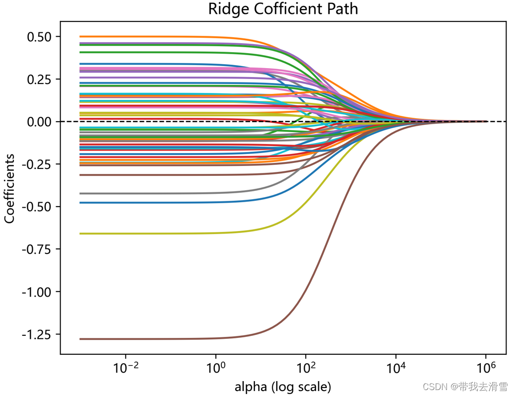
（6）考虑惩罚参数的网格np.logspace(-3，6，100)，画出岭回归的系数路径

plt.rcParams['font.sans-serif']=['Microsoft YaHei']

model = Ridge()#拟合模型
model.fit(X, y)#计算测试集上的拟合优度
model.score(X, y)#模型截距
model.intercept_#模型系数
model.coef_#数据框展示系数
pd.DataFrame(model.coef_, index=X_raw.columns, columns=['Coefficient'])

alphas = np.logspace(-3, 6, 100)
coefs = []
for alpha in alphas:
    model = Ridge(alpha=alpha)
    model.fit(X, y)
    coefs.append(model.coef_) 
ax = plt.gca()
ax.plot(alphas, coefs)
ax.set_xscale('log')#将横轴尺度改为对数尺度
plt.xlabel('alpha (log scale)')#设置纵轴名称
plt.ylabel('Coefficients')#横轴名称
plt.title('Ridge Cofficient Path')#设置标题名称
plt.axhline(0, linestyle='--', linewidth=1, color='k')#添加线条颜色、宽度、样式
plt.savefig("squares8.png",
            bbox_inches ="tight",
            pad_inches = 0.5,
            transparent = True,
            facecolor ="w",
            edgecolor ='w',
            dpi=300,
            orientation ='landscape')#保存高清图片

输出结果：

 

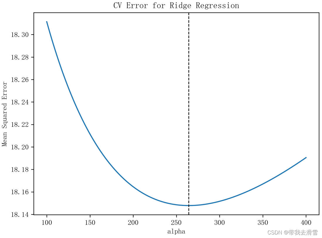
 （7）通过10折交叉验证（使用random-state=1），选择最优惩罚参数，进行岭回归，以数据框的形式展示最优岭回归的系数，并画出交叉验证图

kfold = KFold(n_splits=10, shuffle=True, random_state=1)
model = RidgeCV(cv=kfold, alphas = np.logspace(-3, 6, 100))
model.fit(X,y)

model.alpha_#最优参数

输出结果：

284.8035868435805

pd.DataFrame(model.coef_, index=X_raw.columns, columns=['Coefficient'])#展示最优岭回归的系数

输出结果：

	Coefficient
age	-0.236550
Medu	0.251025
Fedu	0.087646
traveltime	-0.124284
studytime	0.229581
failures	-0.726786
famrel	0.114305
freetime	0.107220
goout	-0.334575
Dalc	-0.078008
Walc	0.010513
health	-0.139548
absences	0.198280
school_GP	-0.030708
school_MS	0.030708
sex_F	-0.208679
sex_M	0.208679
address_R	-0.093834
address_U	0.093834
famsize_GT3	-0.120611
famsize_LE3	0.120611
Pstatus_A	0.061713
Pstatus_T	-0.061713
Mjob_at_home	-0.064841
Mjob_health	0.192810
Mjob_other	-0.132952
Mjob_services	0.174610
Mjob_teacher	-0.124117
Fjob_at_home	0.010097
Fjob_health	0.061756
Fjob_other	-0.084339
Fjob_services	-0.049912
Fjob_teacher	0.189040
reason_course	-0.132146
reason_home	-0.069339
reason_other	0.128259
reason_reputation	0.130782
guardian_father	0.016487
guardian_mother	-0.002703
guardian_other	-0.020767
schoolsup_no	0.159480
schoolsup_yes	-0.159480
famsup_no	0.144278
famsup_yes	-0.144278
paid_no	-0.085224
paid_yes	0.085224
activities_no	0.044861
activities_yes	-0.044861
nursery_no	0.014338
nursery_yes	-0.014338
higher_no	-0.171359
higher_yes	0.171359
internet_no	-0.082825
internet_yes	0.082825
romantic_no	0.188334
romantic_yes	-0.188334

        通过10折交叉验证，可以发现最优惩罚参数为284.8035868435805，介于100到400之间，下面我们将100到400这个区间等分成10000份，并画出交叉验证图。

alphas = np.linspace(100,400,10000)
kfold = KFold(n_splits=10, shuffle=True, random_state=1)
model=RidgeCV( alphas = alphas,store_cv_values=True)#store_cv_values=True表示保留交叉验证结果，方便后续画交叉验证图
model.fit(X,y)
model.alpha_#最优参数
model.cv_values_.shape
mse = np.mean(model.cv_values_, axis=0)
np.min(mse)
 
index_min = np.argmin(mse)
print(index_min)
 
alphas[index_min], mse[index_min]
 
plt.plot(alphas, mse)
plt.axvline(alphas[index_min], linestyle='--', linewidth=1, color='k')
plt.xlabel('alpha')
plt.ylabel('Mean Squared Error')
plt.title('CV Error for Ridge Regression')
plt.tight_layout()

plt.savefig("squares9.png",
            bbox_inches ="tight",
            pad_inches = 0.5,
            transparent = True,
            facecolor ="w",
            edgecolor ='w',
            dpi=300,
            orientation ='landscape')

输出结果：

 

（8）设定参数“eps=le-4”，使用lasso_path()函数，画出lasso回归的系数路径

model = Lasso(alpha=0.1)#设置lasso惩罚回归参数为alpha为0.1，默认值是1
model.fit(X, y)
model.score(X, y)
results = pd.DataFrame(model.coef_, index=X_raw.columns, columns=['Coefficient'])
results
输出结果：

	Coefficient
age	-2.111173e-01
Medu	2.866335e-01
Fedu	0.000000e+00
traveltime	-9.388186e-02
studytime	2.717281e-01
failures	-1.239859e+00
famrel	7.466518e-02
freetime	1.428622e-01
goout	-4.529076e-01
Dalc	-0.000000e+00
Walc	0.000000e+00
health	-1.500360e-01
absences	2.742405e-01
school_GP	-0.000000e+00
school_MS	0.000000e+00
sex_F	-4.526523e-01
sex_M	5.396527e-17
address_R	-1.360996e-01
address_U	0.000000e+00
famsize_GT3	-2.187237e-01
famsize_LE3	0.000000e+00
Pstatus_A	5.153623e-02
Pstatus_T	-1.259190e-16
Mjob_at_home	0.000000e+00
Mjob_health	3.575497e-01
Mjob_other	-0.000000e+00
Mjob_services	3.937326e-01
Mjob_teacher	-5.542350e-02
Fjob_at_home	0.000000e+00
Fjob_health	4.590915e-02
Fjob_other	-2.621918e-02
Fjob_services	-0.000000e+00
Fjob_teacher	2.370666e-01
reason_course	-7.803347e-02
reason_home	-0.000000e+00
reason_other	1.145961e-01
reason_reputation	1.217747e-01
guardian_father	0.000000e+00
guardian_mother	-0.000000e+00
guardian_other	0.000000e+00
schoolsup_no	3.257447e-01
schoolsup_yes	-3.237916e-16
famsup_no	2.804992e-01
famsup_yes	-0.000000e+00
paid_no	-6.048454e-02
paid_yes	0.000000e+00
activities_no	4.667755e-02
activities_yes	-0.000000e+00
nursery_no	0.000000e+00
nursery_yes	-0.000000e+00
higher_no	-2.443272e-01
higher_yes	8.994212e-16
internet_no	-9.205186e-02
internet_yes	5.396527e-17
romantic_no	3.797759e-01
romantic_yes	-0.000000e+00

 plt.rcParams['font.sans-serif']=['Microsoft YaHei']#保证负号正常显示
alphas, coefs, _ = lasso_path(X, y, eps=1e-4)#画出lasso回归的系数路径
ax = plt.gca()
ax.plot(alphas, coefs.T)
ax.set_xscale('log')
plt.xlabel('alpha (log scale)')
plt.ylabel('Coefficients')
plt.title('Lasso Cofficient Path')
plt.axhline(0, linestyle='--', linewidth=1, color='k')
plt.savefig("squares10.png",
            bbox_inches ="tight",
            pad_inches = 0.5,
            transparent = True,
            facecolor ="w",
            edgecolor ='w',
            dpi=300,
            orientation ='landscape')

输出结果：

 

（9）通过10折交叉验证（使用random-state=1），在网格np.logspace(-3，1，100)上选择最优惩罚参数，进行Lasso回归，并以数据框的形式展示最优Lasso回归的系数

kfold = KFold(n_splits=10, shuffle=True, random_state=1)
alphas=np.logspace(-3, 1, 100)
model = LassoCV(alphas=alphas, cv=kfold)
model.fit(X, y)
model.alpha_   
 
pd.DataFrame(model.coef_, index=X_raw.columns, columns=['Coefficient'])

输出结果：

	Coefficient
age	-1.335234e-01
Medu	3.037488e-01
Fedu	0.000000e+00
traveltime	-7.782359e-02
studytime	1.608208e-01
failures	-1.239094e+00
famrel	7.038920e-03
freetime	3.799272e-02
goout	-3.502907e-01
Dalc	-0.000000e+00
Walc	0.000000e+00
health	-6.823233e-02
absences	1.547020e-01
school_GP	-0.000000e+00
school_MS	0.000000e+00
sex_F	-3.598980e-01
sex_M	1.079305e-16
address_R	-9.641718e-02
address_U	0.000000e+00
famsize_GT3	-1.640174e-01
famsize_LE3	0.000000e+00
Pstatus_A	9.131875e-03
Pstatus_T	-7.195369e-17
Mjob_at_home	-0.000000e+00
Mjob_health	2.895078e-01
Mjob_other	-0.000000e+00
Mjob_services	3.410783e-01
Mjob_teacher	-0.000000e+00
Fjob_at_home	0.000000e+00
Fjob_health	0.000000e+00
Fjob_other	-0.000000e+00
Fjob_services	-0.000000e+00
Fjob_teacher	1.367522e-01
reason_course	-1.042161e-01
reason_home	-0.000000e+00
reason_other	4.090333e-02
reason_reputation	5.860171e-02
guardian_father	0.000000e+00
guardian_mother	-0.000000e+00
guardian_other	0.000000e+00
schoolsup_no	2.318489e-01
schoolsup_yes	-2.518379e-16
famsup_no	1.753731e-01
famsup_yes	-0.000000e+00
paid_no	-0.000000e+00
paid_yes	0.000000e+00
activities_no	0.000000e+00
activities_yes	-0.000000e+00
nursery_no	0.000000e+00
nursery_yes	-0.000000e+00
higher_no	-1.939954e-01
higher_yes	7.195369e-17
internet_no	-5.816817e-02
internet_yes	0.000000e+00
romantic_no	3.038162e-01
romantic_yes	-0.000000e+00

（10）考虑惩罚参数的网格np.logspace(-3，1，100)与调节参数11_ratio的网格[0.001，0.01，0.1，0.5，1]，并通过10折交叉验证（使用random-state=1）,选择最优参数与11_ratio，进行弹性网回归，汇报样本内的拟合优度，并以数据框的形式展示最优弹性网回归的系数

alphas = np.logspace(-3, 1, 100)
kfold = KFold(n_splits=10, shuffle=True, random_state=1)
model = ElasticNetCV(cv=kfold, alphas = alphas, l1_ratio=[0.0001, 0.001, 0.01, 0.1, 0.5, 1])
model.fit(X,y)

model.alpha_#最优alpha

输出结果：

0.7390722033525783

model.l1_ratio_#一范数的比例

输出结果：

0.0001

model.score(X,y)#拟合优度

输出结果：

0.2386472416638149

pd.DataFrame(model.coef_, index=X_raw.columns, columns=['Coefficient'])#变量系数

输出结果：

	Coefficient
age	-0.234207
Medu	0.249271
Fedu	0.088374
traveltime	-0.123689
studytime	0.226776
failures	-0.719687
famrel	0.113137
freetime	0.105266
goout	-0.330888
Dalc	-0.077127
Walc	0.008907
health	-0.138091
absences	0.195197
school_GP	-0.029868
school_MS	0.029867
sex_F	-0.206908
sex_M	0.206907
address_R	-0.093429
address_U	0.093429
famsize_GT3	-0.119904
famsize_LE3	0.119903
Pstatus_A	0.061574
Pstatus_T	-0.061574
Mjob_at_home	-0.065240
Mjob_health	0.191109
Mjob_other	-0.132072
Mjob_services	0.172806
Mjob_teacher	-0.121191
Fjob_at_home	0.009670
Fjob_health	0.061303
Fjob_other	-0.083404
Fjob_services	-0.049209
Fjob_teacher	0.186866
reason_course	-0.131521
reason_home	-0.068707
reason_other	0.127367
reason_reputation	0.130086
guardian_father	0.016938
guardian_mother	-0.002386
guardian_other	-0.021881
schoolsup_no	0.158340
schoolsup_yes	-0.158340
famsup_no	0.143039
famsup_yes	-0.143039
paid_no	-0.084988
paid_yes	0.084988
activities_no	0.044180
activities_yes	-0.044180
nursery_no	0.013812
nursery_yes	-0.013812
higher_no	-0.171041
higher_yes	0.171041
internet_no	-0.082580
internet_yes	0.082580
romantic_no	0.187161
romantic_yes	-0.187161

       可以发现，进行弹性网回归，通过10折交叉验证,最优参数的值为0.7390722033525783，11_ratio的值为0.0001，样本内的拟合优度为0.2386472416638149。

（11）使用random-state=0，随机预留100个观测值作为测试集，进行最优的弹性网回归，分别计算训练集与测试集的拟合优度

X_train, X_test, y_train, y_test = train_test_split(X, y, test_size=0.25, random_state=0)
alphas = np.logspace(-3, 1, 100)
kfold = KFold(n_splits=10, shuffle=True, random_state=1)
model = ElasticNetCV(cv=kfold, alphas = alphas, l1_ratio=[0.0001, 0.001, 0.01, 0.1, 0.5, 1])
model.fit(X_train, y_train)
model.alpha_
model.score(X_train, y_train)#训练集拟合优度

model.score(X_test, y_test)#测试集拟合优度

参考资料： 陈强.机器学习及Python应用. 北京：高等教育出版社, 2021.

---

需要数据集的家人们可以去百度网盘（永久有效）获取：

链接：https://pan.baidu.com/s/1bkMo4oCAZYud1Dcu1upu_w?pwd=cori 
提取码：cori 
--来自百度网盘超级会员V5的分享

---

更多优质内容持续发布中，请移步主页查看。

   点赞+关注,下次不迷路！