


大家好,我是带我去滑雪!
决策树模型可以处理各种类型的特征(连续型、离散型、类别型等),不需要对特征进行过多的预处理工作,因此非常适合初步探索数据。通过绘制混淆矩阵、ROC曲线和特征变量重要性排序图,可以直观地了解模型的性能表现以及对于预测的重要特征,有助于进一步分析和改进模型。下面开始代码实战。
目录
(1)导入相关模块
import matplotlib.pyplot as plt
import numpy as np
import pandas as pd
from sklearn import tree
import seaborn as sns
from sklearn.metrics import recall_score
from sklearn.metrics import precision_score
from sklearn.metrics import f1_score
from sklearn.model_selection import train_test_split
(2)导入数据
data = pd.read_csv(r'E:\工作\硕士\博客\博客粉丝问题\data.csv',encoding="utf-8")
data = data.fillna(-1)#补全数据
print(data)
#划分训练集和验证集
y=data.iloc[:,-1]
print(y)
X=data.iloc[:,:-1]
输出结果:
geologic structure  human activity  underground water  susceptibility
0                     0               1                  1               1
1                     0               1                  1               1
2                     0               1                  1               1
3                     0               0                  1               1
4                     0               1                  1               1
..                  ...             ...                ...             ...
207                   1               1                  1               1
208                   1               1                  0               1
209                   1               1                  1               1
210                   0               1                  0               1
211                   1               1                  1               1

[212 rows x 4 columns]
0      1
1      1
2      1
3      1
4      1
      ..
207    1
208    1
209    1
210    1
211    1
Name: susceptibility, Length: 212, dtype: int64
(3)数据标准化与决策树模型构建
from sklearn.model_selection import train_test_split
X_train, X_test, y_train, y_test =  train_test_split(X,y,test_size = 0.25, random_state= 0)
from sklearn.preprocessing import StandardScaler
scaler = StandardScaler()
scaler.fit(X_train)
X_train = scaler.transform(X_train)
X_test= scaler.transform(X_test)
print('训练数据形状:')
print(X_train.shape,y_train.shape)
print('验证测试数据形状:')
(X_test.shape,y_test.shape)
print(y_test)


from sklearn.tree import DecisionTreeClassifier
classifier = DecisionTreeClassifier()
classifier = classifier.fit(X_train,y_train)
#prediction
y_pred = classifier.predict(X_test)#Accuracy
from sklearn import metrics
print('Accuracy Score:', metrics.accuracy_score(y_test,y_pred))
from sklearn.metrics import confusion_matrix
cm = confusion_matrix(y_test, y_pred)
cm
输出结果:
Accuracy Score: 0.6792452830188679array([[17, 6], [11, 19]], dtype=int64)
(4)绘制混淆矩阵
from sklearn import metrics
cm = metrics.confusion_matrix(penguin_tree.predict(X_test), y_test)
plt.figure()
sns.heatmap(cm , annot=True, cmap='Blues')
plt.xlabel('Predicted labels')
plt.ylabel('True labels')
plt.savefig(r'E:\工作\硕士\博客\博客粉丝问题\决策树混淆矩阵.png',
            bbox_inches ="tight",
            pad_inches = 1,
            transparent = True,
            facecolor ="w",
            edgecolor ='w',
            dpi=300,
            orientation ='landscape')

pred=y_pred
pred = classifier.predict(X_test)
pred[:5]
(5)计算决策树模型的准确度、精度、召回率、F1度量
from sklearn import metrics
import numpy as np
import pandas as pd
import matplotlib.pyplot as plt
%matplotlib inline

from sklearn.datasets import load_iris
from sklearn.model_selection import train_test_split
from sklearn.tree import DecisionTreeClassifier
from sklearn.metrics import cohen_kappa_score
from sklearn.metrics import confusion_matrix
from sklearn.metrics import classification_report
print("决策树模型在测试集上的准确度为:", metrics.accuracy_score(pred, y_test))
print("决策树模型在测试集上的精度为:", metrics.average_precision_score(pred, y_test))
print("决策树模型在测试集上的召回率为:", metrics.recall_score(pred, y_test))
print("决策树模型在测试集上的F1度量为:", metrics.f1_score(pred, y_test))
输出结果:
树模型在测试集上的准确度为: 0.6792452830188679
树模型在测试集上的精度为: 0.5945408805031447
树模型在测试集上的召回率为: 0.76
树模型在测试集上的F1度量为: 0.6909090909090909
(6)参数寻优
parameters = {'splitter':('best','random')
                ,'criterion':("gini","entropy")
                ,"max_depth":[*range(1,10)]
                ,'min_samples_leaf':[*range(1,50,5)]
                ,'min_impurity_decrease':[*np.linspace(0,0.5,20)]
}
classifier = DecisionTreeClassifier(random_state=25)
GS = GridSearchCV(classifier, parameters, cv=10)
GS.fit(X_train,y_train)
print(GS.best_params_)
print(GS.best_score_)
输出结果:
{'criterion': 'gini', 'max_depth': 3, 'min_impurity_decrease': 0.0, 'min_samples_leaf': 1, 'splitter': 'best'}
0.7358333333333333
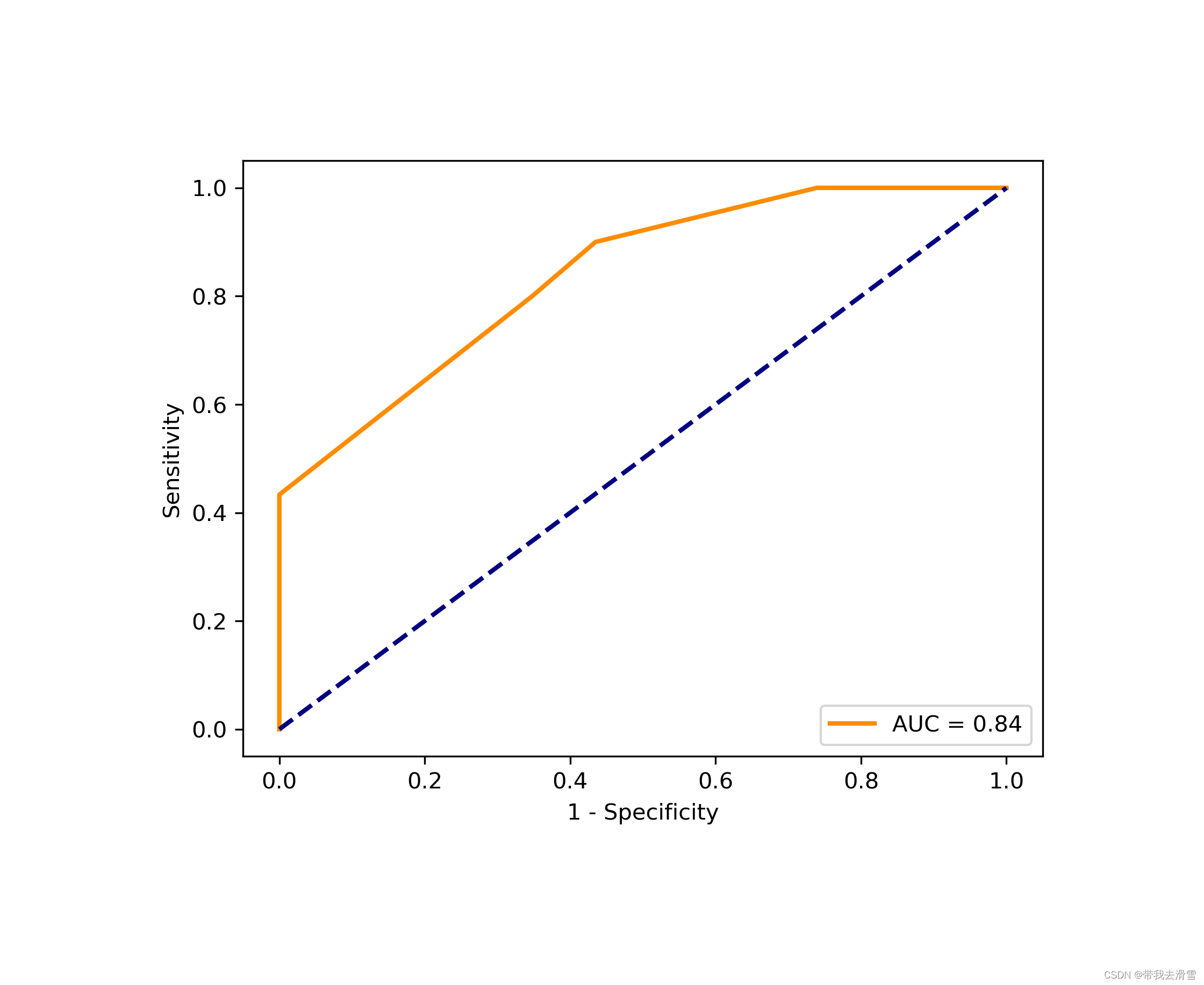
(7)绘制ROC曲线
 import sklearn.metrics as metrics
y_pred_clf = clf.predict_proba(X_test)[:,1]
fpr, tpr, threshold=metrics.roc_curve(y_test,y_pred_clf)
roc_auc = metrics.auc(fpr, tpr)
#plt.plot(fpr, tpr, 'b', label='AUC = %0.2f' % roc_auc)#生成ROC曲线
lw = 2
plt.plot(fpr, tpr, color='darkorange',lw=lw, label='AUC = %0.2f' % roc_auc)  ###假正率为横坐标,真正率为纵坐标做曲线
plt.plot([0, 1], [0, 1], color='navy', lw=lw, linestyle='--')
plt.xlim([-0.05, 1.05])
plt.ylim([-0.05, 1.05])
plt.xlabel('1 - Specificity')
plt.ylabel('Sensitivity')
# plt.title('ROCs for Densenet')
plt.legend(loc="lower right")

plt.savefig(r'E:\工作\硕士\博客\博客粉丝问题\决策树ROC曲线.png',
            bbox_inches ="tight",
            pad_inches = 1,
            transparent = True,
            facecolor ="w",
            edgecolor ='w',
            dpi=300,
            orientation ='landscape')
输出结果:
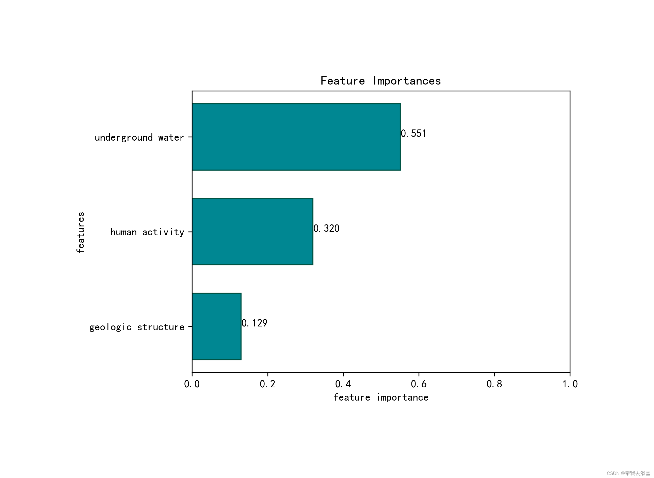
(8)绘制模型的特征变量重要性排序图
features_import = pd.DataFrame(X_train.columns, columns=['feature'])
features_import['importance'] =classifier.feature_importances_  # 默认按照gini计算特征重要性
features_import.sort_values('importance', inplace=True)
# 绘图
from matplotlib import pyplot as plt
plt.rcParams['font.sans-serif'] = ['SimHei']  # 显示中文黑体
# plt.rcParams['axes.unicode_minus'] = False # 负值显示
plt.barh(features_import['feature'], features_import['importance'], height=0.7, color='#008792', edgecolor='#005344') # 更多颜色可参见颜色大全
plt.xlabel('feature importance') # x 轴
plt.ylabel('features') # y轴
plt.xlim(0,1)
plt.title('Feature Importances') # 标题
for a,b in zip( features_import['importance'],features_import['feature']): # 添加数字标签
    print(a,b)
    plt.text(a+0.001, b,'%.3f'%float(a)) # a+0.001代表标签位置在柱形图上方0.001处

plt.savefig(r'E:\工作\硕士\博客\博客粉丝问题\决策树变量重要性程度.png',
            bbox_inches ="tight",
            pad_inches = 1,
            transparent = True,
            facecolor ="w",
            edgecolor ='w',
            dpi=300,
            orientation ='landscape')
输出结果:
需要数据集的家人们可以去百度网盘(永久有效)获取:
链接:https://pan.baidu.com/s/173deLlgLYUz789M3KHYw-Q?pwd=0ly6
提取码:2138
更多优质内容持续发布中,请移步主页查看。
若有问题可邮箱联系:1736732074@qq.com
博主的WeChat:TCB1736732074
点赞+关注,下次不迷路!


 6348
6348


 被折叠的 条评论
为什么被折叠?
被折叠的 条评论
为什么被折叠?
 到【灌水乐园】发言


