


code
- 正则化
import numpy as np
import h5py
import matplotlib.pyplot as plt
from dnn_utils_v2 import *
from load_data import load_2D_dataset
class dnn:
def __init__(self,layer_dims) -> None:
self.WL={}
self.bL={}
self.L=len(layer_dims)-1
np.random.seed(3)
# 初始化参数
for i in range(1,self.L+1):
self.WL['W'+str(i)]=np.random.randn(layer_dims[i], layer_dims[i-1]) / np.sqrt(layer_dims[i-1])
self.bL['b'+str(i)]=np.zeros((layer_dims[i],1))
self.XL={}
self.AL={}
self.ZL={}
self.dZ={}
self.dW={}
self.db={}
self.dA={}
def input_data(self,X,Y,learning_rate):
self.m=X.shape[1]
self.AL["A0"]=X
self.Y=Y
self.learning_rate=learning_rate
def set_data(self,X):
self.m=X.shape[1]
self.AL["A0"]=X
#下面是前向传播模块,前向传播过程中需要记录Z,A
def linear_activation_forward(self,i,activation):
'''实现一层的正向传播'''
# self.ZL[Zi]和self.AL[Ai]记录第i层的数据
# 存储了计算的Z ,A,W,b,对象自带的有
self.ZL['Z'+str(i)]=np.dot(self.WL['W'+str(i)],self.AL['A'+str(i-1)])+self.bL['b'+str(i)]
if activation=="sigmoid":
self.AL['A'+str(i)]=1/(1+np.exp(-self.ZL['Z'+str(i)]))
elif activation=="relu":
self.AL['A'+str(i)]=np.maximum(0,self.ZL['Z'+str(i)])
def L_model_forward(self):
# 前L-1层使用relu函数激活,最后一层使用sigmoid函数激活
for i in range(1,self.L):
self.linear_activation_forward(i,"relu")
self.linear_activation_forward(self.L,"sigmoid")
# 确定最后的输出是否是二分类所需要的输出
assert(self.AL['A'+str(self.L)].shape==(1,self.m))
# 下面是计算损失函数
# 无正则化损失函数
def computer_cost(self):
return np.squeeze(-1/self.m*np.sum(self.Y*np.log(self.AL['A'+str(self.L)])+(1-self.Y)*np.log(1-self.AL['A'+str(self.L)])))
# 含有正则化的损失函数
def computer_cost_regularization(self,lambd):
'''lambd正则化参数'''
# 计算正则化项
regularzation=0
for i in range(1,self.L+1):
regularzation+=np.sum(np.square(self.WL['W'+str(i)]))
return self.computer_cost()+lambd/(2*self.m)*regularzation
# 下面是反向传播模块
# 无正则化线性的反向传播
def linear_backward(self,i):
'''根据dz[L]计算dw[L],db[L],dA[L-1]'''
self.dW['dW'+str(i)]=1/self.m*np.dot(self.dZ['dZ'+str(i)],self.AL["A"+str(i-1)].T)
self.db['db'+str(i)]=1/self.m*np.sum(self.dZ['dZ'+str(i)],axis=1,keepdims=True)
self.dA['dA'+str(i-1)]=np.dot(self.WL['W'+str(i)].T,self.dZ['dZ'+str(i)])
# 有正则化的线性反向传播
def linear_backward_regularization(self,i,lambd):
self.dW['dW'+str(i)]=1/self.m*np.dot(self.dZ['dZ'+str(i)],self.AL["A"+str(i-1)].T)+lambd/self.m*self.WL["W"+str(i)]
self.db['db'+str(i)]=1/self.m*np.sum(self.dZ['dZ'+str(i)],axis=1,keepdims=True)
self.dA['dA'+str(i-1)]=np.dot(self.WL['W'+str(i)].T,self.dZ['dZ'+str(i)])
def L_model_backforward(self):
# 先计算最后一层
# 计算dA
self.dA['dA'+str(self.L)]=-(np.divide(self.Y,self.AL['A'+str(self.L)])-np.divide(1-self.Y,1-self.AL['A'+str(self.L)]))
# 计算dz
s=1/(1+np.exp(-self.ZL['Z'+str(self.L)]))
self.dZ['dZ'+str(self.L)]=self.dA['dA'+str(self.L)]*s*(1-s)
# 计算dw,db,dA[L-1]
self.linear_backward(self.L)
for i in reversed(range(self.L)):
if i==0:
break
else:
self.dZ['dZ'+str(i)]=relu_backward(self.dA['dA'+str(i)],self.ZL['Z'+str(i)])
# 计算当前i层的dw,db,和dA[L-1]
self.linear_backward(i)
def L_model_backforward_regularization(self,lambd):
# 计算最后最后一层的dA
self.dA['dA'+str(self.L)]=-(np.divide(self.Y,self.AL['A'+str(self.L)])-np.divide(1-self.Y,1-self.AL['A'+str(self.L)]))
# 计算dz
s=1/(1+np.exp(-self.ZL['Z'+str(self.L)]))
self.dZ['dZ'+str(self.L)]=self.dA['dA'+str(self.L)]*s*(1-s)
# 计算dw,wb,dA[L-1]
self.linear_backward_regularization(self.L,lambd)
for i in reversed(range(self.L)):
if i==0:
break
else:
self.dZ['dZ'+str(i)]=relu_backward(self.dA['dA'+str(i)],self.ZL['Z'+str(i)])
self.linear_backward_regularization(i,lambd)
# 更新参数
def update_wb(self):
for i in range(1,self.L+1):
self.WL['W'+str(i)]=self.WL['W'+str(i)]-self.learning_rate*self.dW['dW'+str(i)]
self.bL['b'+str(i)]=self.bL['b'+str(i)]-self.learning_rate*self.db['db'+str(i)]
def train(self,iterations,lambd=0,flag=0):
costs=[]
if flag==0:
# 说明不使用正则
print("非正则化")
for i in range(iterations):
# 前向传播
self.L_model_forward()
# 计算损失
cost=self.computer_cost()
# 后向传播
self.L_model_backforward()
# 更新参数
self.update_wb()
if i%1000==0:
costs.append(cost)
print("第"+str(i)+"次迭代cost:"+str(cost))
else:
# 使用正则
print("正则化")
for i in range(iterations):
# 前向传播
self.L_model_forward()
# 计算损失
cost=self.computer_cost_regularization(lambd)
# 后向传播
self.L_model_backforward_regularization(lambd)
# 更新参数
self.update_wb()
if i%1000==0:
costs.append(cost)
print("第"+str(i)+"次迭代cost:"+str(cost))
return costs
def predict(self,X):
self.set_data(X)
self.L_model_forward()
ans=np.zeros((self.AL['A'+str(self.L)].shape[0],self.AL['A'+str(self.L)].shape[1]))
for i in range(0,self.AL['A'+str(self.L)].shape[1]):
if(self.AL['A'+str(self.L)][0,i]>0.5):
ans[0,i]=1
return ans
#加载数据
train_x, train_y, test_x, test_y = load_2D_dataset()
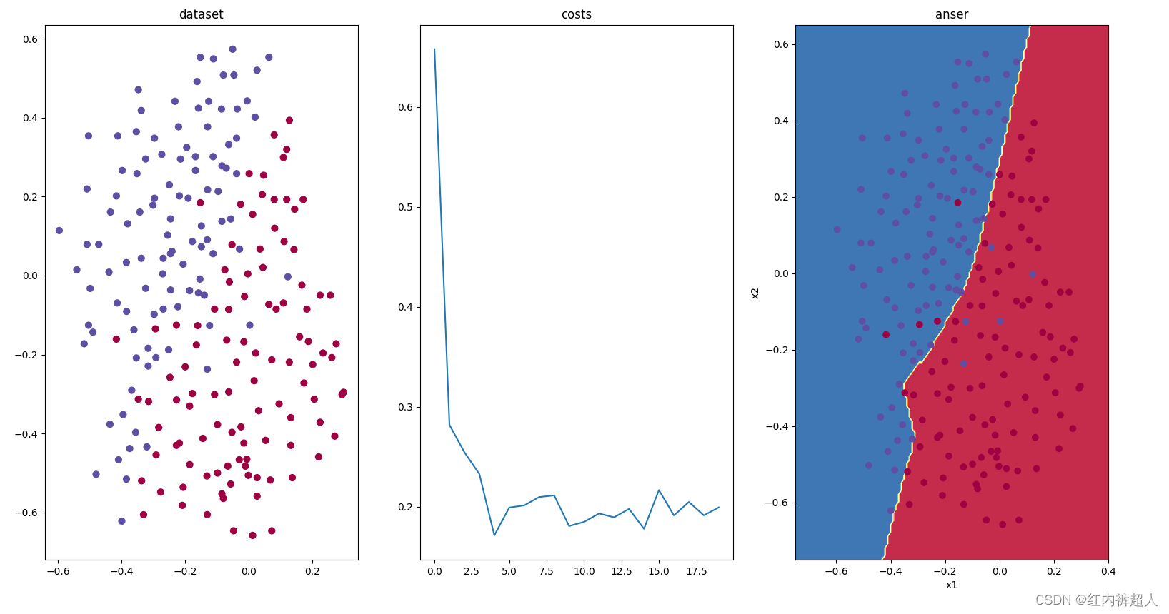
plt.subplot(1,3,1)
plt.title("dataset")
plt.scatter(train_x[0, :], train_x[1, :], c=train_y, s=40, cmap=plt.cm.Spectral)
# # 4层的神经网络
my_dnn=dnn([train_x.shape[0], 20, 3, 1])
my_dnn.input_data(train_x,train_y,0.3 )
print("开始训练")
# 正则化
# costs=my_dnn.train(20000,0.7,1)
# 无正则化
costs=my_dnn.train(20000,0,0)
print("训练结束")
# 画损失曲线图
plt.subplot(1,3,2)
plt.title("costs")
plt.plot(costs)
# 画分类图
plt.subplot(1,3,3)
plt.title("anser")
axes = plt.gca()
axes.set_xlim([-0.75,0.40])
axes.set_ylim([-0.75,0.65])
plot_decision_boundary(lambda x: my_dnn.predict(x.T), train_x, train_y)
y_predict_train=my_dnn.predict(train_x)
y_predict_test=my_dnn.predict(test_x)
# 准确率
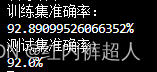
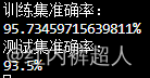
print("训练集准确率:")
print(str((1-np.sum(np.abs(y_predict_train-train_y))/train_y.shape[1])*100)+"%")
print("测试集准确率:")
print(str((1-np.sum(np.abs(y_predict_test-test_y))/test_y.shape[1])*100)+"%")
plt.show()
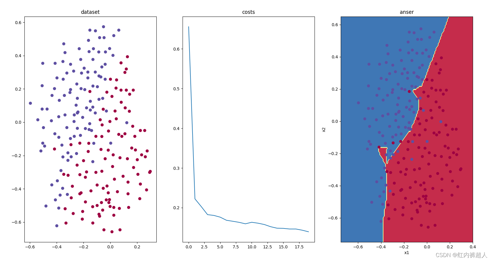
非正则化训练20000,学习率0.3的训练结果
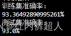
L2正则化训练20000,学习率0.3,lambda0.7的训练结果
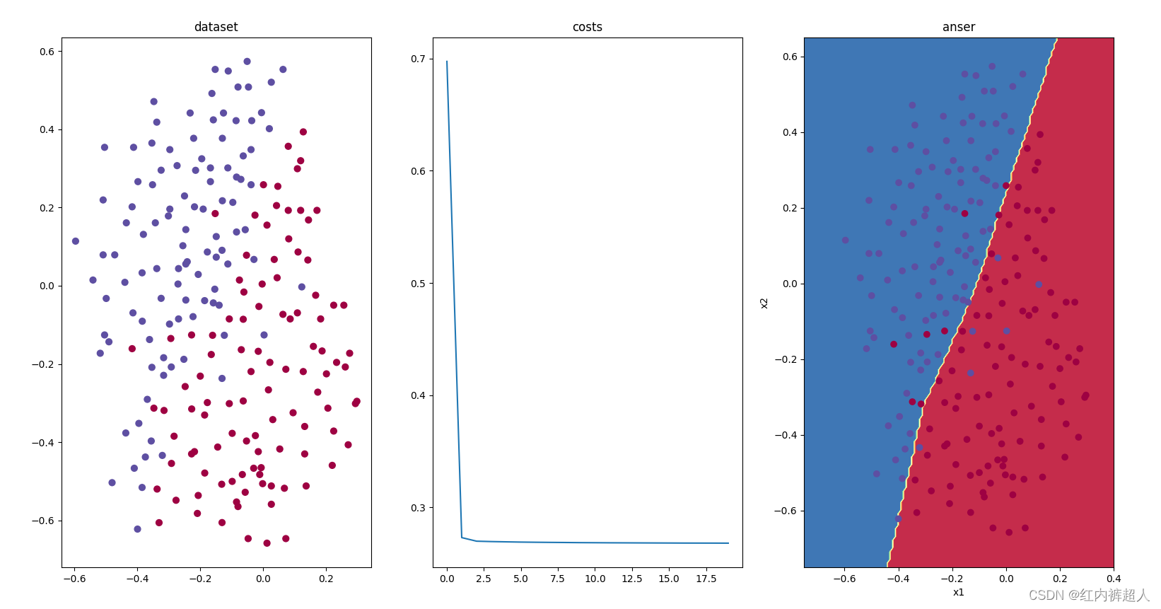
实验结果:
第二个实验的方差减小,说明L2正则化对降低过拟合(高方差)有效。
- dropout
code
import numpy as np
import h5py
import matplotlib.pyplot as plt
from dnn_utils_v2 import  *
from load_data import load_2D_dataset
class dnn:
    def __init__(self,layer_dims) -> None:

        self.WL={}
        self.bL={}
        self.L=len(layer_dims)-1
        np.random.seed(3)
        # 初始化参数
        for i in range(1,self.L+1):
            self.WL['W'+str(i)]=np.random.randn(layer_dims[i], layer_dims[i-1]) / np.sqrt(layer_dims[i-1])
            self.bL['b'+str(i)]=np.zeros((layer_dims[i],1))
        self.XL={}
        self.AL={}
        self.ZL={}
        self.dZ={}
        self.dW={}
        self.db={}
        self.dA={}
        # dropout所用到的参数
        self.do={}
    def input_data(self,X,Y,learning_rate):
        self.m=X.shape[1]
        self.AL["A0"]=X
        self.Y=Y
        self.learning_rate=learning_rate
    def set_data(self,X):
        self.m=X.shape[1]
        self.AL["A0"]=X
    #下面是前向传播模块,前向传播过程中需要记录Z,A
    # 无dropout的前向传播
    def linear_activation_forward(self,i,activation):
        '''实现一层的正向传播'''
        # self.ZL[Zi]和self.AL[Ai]记录第i层的数据
        # 存储了计算的Z ,A,W,b,对象自带的有
        self.ZL['Z'+str(i)]=np.dot(self.WL['W'+str(i)],self.AL['A'+str(i-1)])+self.bL['b'+str(i)]
        if activation=="sigmoid":
            self.AL['A'+str(i)]=1/(1+np.exp(-self.ZL['Z'+str(i)]))
        elif activation=="relu":
            self.AL['A'+str(i)]=np.maximum(0,self.ZL['Z'+str(i)])
    # 有dropout前向传播
    def linear_activation_forward_dropout(self,i,activation,keep_prob):
        self.ZL['Z'+str(i)]=np.dot(self.WL['W'+str(i)],self.AL['A'+str(i-1)])+self.bL['b'+str(i)]
        if activation=="sigmoid":
            self.AL['A'+str(i)]=1/(1+np.exp(-self.ZL['Z'+str(i)]))
        elif activation=="relu":
            self.AL['A'+str(i)]=np.maximum(0,self.ZL['Z'+str(i)])
        # 随机dropout
        self.do['do'+str(i)]=np.random.rand(self.AL['A'+str(i)].shape[0],self.AL['A'+str(i)].shape[1])
        # 输出层不应用dropout
        if i!=self.L:
            self.do['do'+str(i)]=self.do['do'+str(i)]<keep_prob  #神经元1-keep_prob的概率失效
            self.AL['A'+str(i)]=self.AL['A'+str(i)]*self.do['do'+str(i)]
            self.AL['A'+str(i)]=self.AL['A'+str(i)]/keep_prob # 缩放

    # 不使用dropout前向传播
    def L_model_forward(self):
        # 前L-1层使用relu函数激活,最后一层使用sigmoid函数激活
        for i in range(1,self.L):
            self.linear_activation_forward(i,"relu")
        self.linear_activation_forward(self.L,"sigmoid")
        # 确定最后的输出是否是二分类所需要的输出
        assert(self.AL['A'+str(self.L)].shape==(1,self.m))
    # 使用dropout的前向传播
    def L_model_forward_dropout(self,keep_prob):
        # 前L-1层使用relu函数激活,最后一层使用sigmoid函数激活
        for i in range(1,self.L):
            self.linear_activation_forward_dropout(i,"relu",keep_prob)
        self.linear_activation_forward_dropout(self.L,"sigmoid",keep_prob)
        # 确定最后的输出是否是二分类所需要的输出
        assert(self.AL['A'+str(self.L)].shape==(1,self.m))

    # 下面是计算损失函数
    def computer_cost(self):
        return np.squeeze(-1/self.m*np.sum(self.Y*np.log(self.AL['A'+str(self.L)])+(1-self.Y)*np.log(1-self.AL['A'+str(self.L)])))

    # 下面是反向传播模块
    def linear_backward(self,i):
        '''根据dz[L]计算dw[L],db[L],dA[L-1]'''
        self.dW['dW'+str(i)]=1/self.m*np.dot(self.dZ['dZ'+str(i)],self.AL["A"+str(i-1)].T)
        self.db['db'+str(i)]=1/self.m*np.sum(self.dZ['dZ'+str(i)],axis=1,keepdims=True)
        self.dA['dA'+str(i-1)]=np.dot(self.WL['W'+str(i)].T,self.dZ['dZ'+str(i)])
    def linear_backward_dropout(self,i,keep_prob):
        self.dW['dW'+str(i)]=1/self.m*np.dot(self.dZ['dZ'+str(i)],self.AL["A"+str(i-1)].T)
        self.db['db'+str(i)]=1/self.m*np.sum(self.dZ['dZ'+str(i)],axis=1,keepdims=True)
        if i==1:
            return
        self.dA['dA'+str(i-1)]=np.dot(self.WL['W'+str(i)].T,self.dZ['dZ'+str(i)])
        self.dA['dA'+str(i-1)]=self.dA['dA'+str(i-1)]* self.do['do'+str(i-1)] # 像正向一样,使用self.do['do'+str(i-1)]关闭同样的神经元
        self.dA['dA'+str(i-1)]=self.dA['dA'+str(i-1)]/keep_prob # 缩放

    def L_model_backforward(self):
        #  先计算最后一层
        # 计算dA
        self.dA['dA'+str(self.L)]=-(np.divide(self.Y,self.AL['A'+str(self.L)])-np.divide(1-self.Y,1-self.AL['A'+str(self.L)]))
        # 计算dz
        s=1/(1+np.exp(-self.ZL['Z'+str(self.L)]))
        self.dZ['dZ'+str(self.L)]=self.dA['dA'+str(self.L)]*s*(1-s)

        # 计算dw,db,dA[L-1]
        self.linear_backward(self.L)
        for i in reversed(range(self.L)):
            if i==0:
                break
            else:
                self.dZ['dZ'+str(i)]=relu_backward(self.dA['dA'+str(i)],self.ZL['Z'+str(i)])
                # 计算当前i层的dw,db,和dA[L-1]
                self.linear_backward(i)

    def L_model_backforward_dropout(self,keep_prob):
        # 计算最后最后一层的dA
        self.dA['dA'+str(self.L)]=-(np.divide(self.Y,self.AL['A'+str(self.L)])-np.divide(1-self.Y,1-self.AL['A'+str(self.L)]))
        # 计算dz
        s=1/(1+np.exp(-self.ZL['Z'+str(self.L)]))
        self.dZ['dZ'+str(self.L)]=self.dA['dA'+str(self.L)]*s*(1-s)
        # 计算dw,wb,dA[L-1]
        self.linear_backward_dropout(self.L,keep_prob)
        for i in reversed(range(self.L)):
            if i==0:
                break
            else:
                self.dZ['dZ'+str(i)]=relu_backward(self.dA['dA'+str(i)],self.ZL['Z'+str(i)])
                self.linear_backward_dropout(i,keep_prob)
    # 更新参数
    def update_wb(self):
        for i in range(1,self.L+1):
            self.WL['W'+str(i)]=self.WL['W'+str(i)]-self.learning_rate*self.dW['dW'+str(i)]
            self.bL['b'+str(i)]=self.bL['b'+str(i)]-self.learning_rate*self.db['db'+str(i)]

    def train(self,iterations,keep_drop=0.5,flag=0):
        costs=[]
        if flag==0:
            # 说明不使用dropout
            print("非dropout")
            for i in range(iterations):
                # 前向传播
                self.L_model_forward()
                # 计算损失
                cost=self.computer_cost()
                # 后向传播
                self.L_model_backforward()
                # 更新参数
                self.update_wb()
                if i%1000==0:
                    costs.append(cost)
                    print("第"+str(i)+"次迭代cost:"+str(cost))
        else:
            # dropout
            print("dropout")
            for i in range(iterations):
                # 前向传播
                self.L_model_forward_dropout(keep_drop)
                # 计算损失
                cost=self.computer_cost()
                # 后向传播
                self.L_model_backforward_dropout(keep_drop)
                # 更新参数
                self.update_wb()
                if i%1000==0:
                    costs.append(cost)
                    print("第"+str(i)+"次迭代cost:"+str(cost))
        return costs
    def predict(self,X):
        self.set_data(X)
        self.L_model_forward()
        ans=np.zeros((self.AL['A'+str(self.L)].shape[0],self.AL['A'+str(self.L)].shape[1]))
        for i in range(0,self.AL['A'+str(self.L)].shape[1]):
            if(self.AL['A'+str(self.L)][0,i]>0.5):
                ans[0,i]=1
        return ans

#加载数据
train_x, train_y, test_x, test_y = load_2D_dataset()

plt.subplot(1,3,1)
plt.title("dataset")
plt.scatter(train_x[0, :], train_x[1, :], c=train_y, s=40, cmap=plt.cm.Spectral)
# # 4层的神经网络
my_dnn=dnn([train_x.shape[0], 20, 3, 1])

my_dnn.input_data(train_x,train_y,0.3 )
print("开始训练")
# dropout
costs=my_dnn.train(20000,0.86,1)
# 无dropout
# costs=my_dnn.train(20000,0,0)
print("训练结束")

# 画损失曲线图
plt.subplot(1,3,2)
plt.title("costs")
plt.plot(costs)

# 画分类图
plt.subplot(1,3,3)
plt.title("anser")
axes = plt.gca()
axes.set_xlim([-0.75,0.40])
axes.set_ylim([-0.75,0.65])
plot_decision_boundary(lambda x: my_dnn.predict(x.T), train_x, train_y)


y_predict_train=my_dnn.predict(train_x)
y_predict_test=my_dnn.predict(test_x)
# 准确率
print("训练集准确率:")
print(str((1-np.sum(np.abs(y_predict_train-train_y))/train_y.shape[1])*100)+"%")
print("测试集准确率:")
print(str((1-np.sum(np.abs(y_predict_test-test_y))/test_y.shape[1])*100)+"%")

plt.show()
dropout:keep_drop=0.86,训练20000


 31
31


 被折叠的 条评论
为什么被折叠?
被折叠的 条评论
为什么被折叠?
 到【灌水乐园】发言


