吴恩达深度学习L2W1作业3

ddancoo

已于 2023-12-07 15:08:59 修改

阅读量860

点赞数 22

文章标签：深度学习人工智能

于 2023-12-07 11:47:34 首次发布

本文链接：https://blog.csdn.net/m0_67611983/article/details/134847674

版权

梯度检验

欢迎来到本周的最后作业！在本作业中，你将学习实现和使用梯度检验。

假设你是致力于在全球范围内提供移动支付的团队的一员，被上级要求建立深度学习模型来检测欺诈行为--每当有人进行支付时，你都应该确认该支付是否可能是欺诈性的，例如用户的帐户已被黑客入侵。

但是模型的反向传播很难实现，有时还会有错误。因为这是关键的应用任务，所以你公司的CEO要反复确定反向传播的实现是正确的。CEO要求你证明你的反向传播实际上是有效的！为了保证这一点，你将应用到“梯度检验”。

让我们开始做吧！

# Packages
import numpy as np
from testCases import *
from gc_utils import sigmoid, relu, dictionary_to_vector, vector_to_dictionary, gradients_to_vector

1 梯度检验原理

反向传播计算梯度 $\frac{\partial J}{\partial \theta }$ ，其中 $\theta$ 表示模型的参数。使用正向传播和损失函数来计算 $\frac{\partial J}{\partial \theta }$ 。

由于正向传播相对容易实现，相信你有信心能做到这一点，确定100％计算正确的损失 $J$ 。为此，你可以使用 $J$ 来验证代码 $\frac{\partial J}{\partial \theta }$ 。

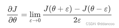
让我们回顾一下导数（或者说梯度）的定义：

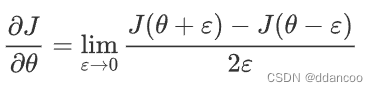
如果你还不熟悉" $\lim_{x\to0 }$ "表示法，其意思只是“当 $\varepsilon$ 值趋向很小时”。

我们知道以下内容：

$\frac{\partial J}{\partial \theta }$ 是你要确保计算正确的对象。
你可以计算 $J(\theta +\varepsilon )$ 和 $J(\theta -\varepsilon )$ 在 $\theta$ 是实数的情况下），因为要保证 $J$ 的实现是正确的。

让我们使用方程式和 $\varepsilon$ 的一个小值来说服CEO你计算 $\frac{\partial J}{\partial \theta }$ 的代码是正确的！

2 一维梯度检查

思考一维线性函数 $J(\theta )=\theta x$ ，该模型仅包含一个实数值参数 $\theta$ ，并以 $x$ 作为输入。

你将实现代码以计算 $J(.)$ 及其派生 $\frac{\partial J}{\partial \theta }$ ，然后，你将使用梯度检验来确保 $J$ 的导数计算正确。

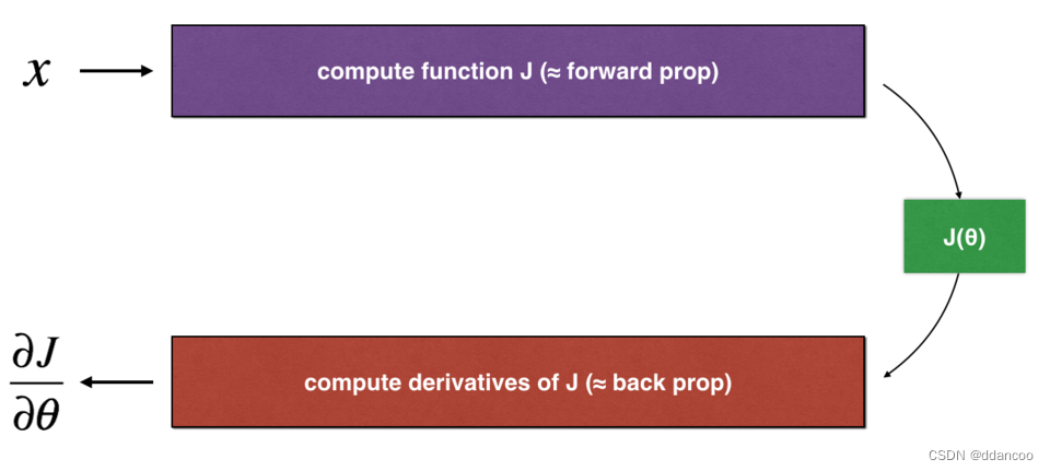
图1：一维线性模型

上图显示了关键的计算步骤：首先从 $x$ 开始，再评估函数 $J(x)$ （正向传播），然后计算导数 $\frac{\partial J}{\partial \theta }$ （反向传播）。

练习：为此简单函数实现“正向传播”和“向后传播”。即在两个单独的函数中，计算 $J(.)$ （正向传播）及其相对于 $\theta$ （反向传播）的导数。

# GRADED FUNCTION: forward_propagation

def forward_propagation(x, theta):
    """
    Implement the linear forward propagation (compute J) presented in Figure 1 (J(theta) = theta * x)
    
    Arguments:
    x -- a real-valued input
    theta -- our parameter, a real number as well
    
    Returns:
    J -- the value of function J, computed using the formula J(theta) = theta * x
    """
    
    ### START CODE HERE ### (approx. 1 line)

    J=theta*x
    ### END CODE HERE ###
    
    return J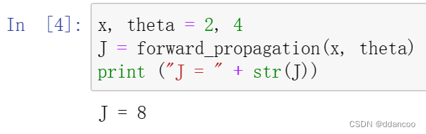

练习：现在，执行图1的反向传播步骤（导数计算）。也就是说，计算 $J(\theta )=\theta x$ 相对于 $\theta$ 的导数。为避免进行演算，你应该得到 $dtheta$ = $\frac{\partial J}{\partial \theta }$ = $x$ 。

# GRADED FUNCTION: backward_propagation

def backward_propagation(x, theta):
    """
    Computes the derivative of J with respect to theta (see Figure 1).
    
    Arguments:
    x -- a real-valued input
    theta -- our parameter, a real number as well
    
    Returns:
    dtheta -- the gradient of the cost with respect to theta
    """
    
    ### START CODE HERE ### (approx. 1 line)

    dtheta=x
    ### END CODE HERE ###
    
    return dtheta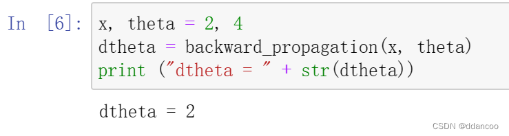

练习：为了展示backward_propagation（）函数正确计算了梯度 $\frac{\partial J}{\partial \theta }$ ，让我们实施梯度检验。

说明：

首先使用上式（1）和 $\varepsilon$ 的极小值计算“gradapprox”。以下是要遵循的步骤：

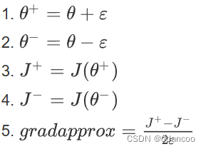
然后使用反向传播计算梯度，并将结果存储在变量“grad”中
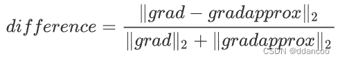
最后，使用以下公式计算“gradapprox”和“grad”之间的相对差：

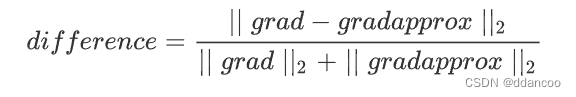
你需要3个步骤来计算此公式：
- 1. 使用np.linalg.norm（...）计算分子
- 2. 计算分母，调用np.linalg.norm（...）两次
- 3. 相除
如果差异很小（例如小于10的-7次方），则可以确信正确计算了梯度。否则，梯度计算可能会出错。

# GRADED FUNCTION: gradient_check

def gradient_check(x, theta, epsilon = 1e-7):
    """
    Implement the backward propagation presented in Figure 1.
    
    Arguments:
    x -- a real-valued input
    theta -- our parameter, a real number as well
    epsilon -- tiny shift to the input to compute approximated gradient with formula(1)
    
    Returns:
    difference -- difference (2) between the approximated gradient and the backward propagation gradient
    """
    
    # Compute gradapprox using left side of formula (1). epsilon is small enough, you don't need to worry about the limit.
    ### START CODE HERE ### (approx. 5 lines)
        # Step 1
    thetaplus=theta+epsilon
        # Step 2
    thetaminus=theta-epsilon
        # Step 3
    J_plus=forward_propagation(x,thetaplus)
        # Step 4
    J_minus=forward_propagation(x,thetaminus)
        # Step 5
    gradapprox=(J_plus-J_minus)/(2*epsilon)    
    ### END CODE HERE ###
        # Check if gradapprox is close enough to the output of backward_propagation()
    ### START CODE HERE ### (approx. 1 line)

    grad=backward_propagation(x,theta)
    ### END CODE HERE ###
    
    ### START CODE HERE ### (approx. 1 line)
        # Step 1'
        # Step 2'
        # Step 3'
    numerator=np.linalg.norm(grad-gradapprox)
    denominator=np.linalg.norm(grad)+np.linalg.norm(gradapprox)
    difference=numerator/denominator
    ### END CODE HERE ###
    
    if difference < 1e-7:
        print ("The gradient is correct!")
    else:
        print ("The gradient is wrong!")
    
    return difference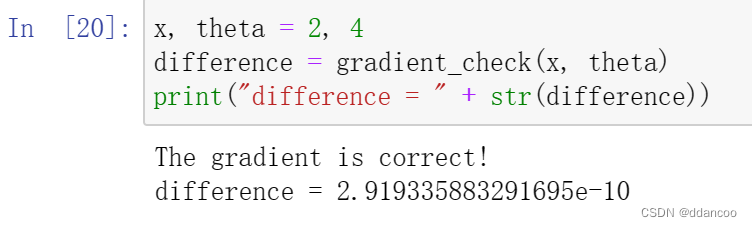

Nice！差异小于阈值10的−7次方。因此可以放心，你已经在backward_propagation（）中正确计算了梯度。

现在，在更一般的情况下，你的损失函数 $J$ 具有多个单个1D输入。当你训练神经网络时， $\theta$ 实际上由多个矩阵 $W^{[l]}$ 组成，并加上偏差 $b^{[l]}$ ！重要的是要知道如何对高维输入进行梯度检验。我们开始动手吧！

3 N维梯度检验

下图描述了欺诈检测模型的正向传播和反向传播：

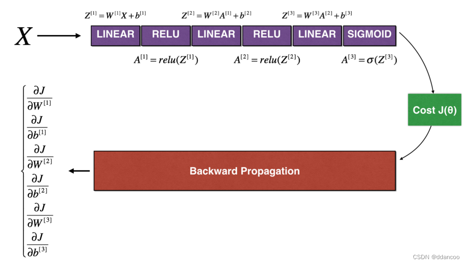
图2：深层神经网络
LINEAR -> RELU -> LINEAR -> RELU -> LINEAR -> SIGMOID

让我们看一下正向传播和反向传播的实现。

def forward_propagation_n(X, Y, parameters):
    """
    Implements the forward propagation (and computes the cost) presented in Figure 3.
    
    Arguments:
    X -- training set for m examples
    Y -- labels for m examples 
    parameters -- python dictionary containing your parameters "W1", "b1", "W2", "b2", "W3", "b3":
                    W1 -- weight matrix of shape (5, 4)
                    b1 -- bias vector of shape (5, 1)
                    W2 -- weight matrix of shape (3, 5)
                    b2 -- bias vector of shape (3, 1)
                    W3 -- weight matrix of shape (1, 3)
                    b3 -- bias vector of shape (1, 1)
    
    Returns:
    cost -- the cost function (logistic cost for one example)
    """
    
    # retrieve parameters
    m = X.shape[1]
    W1 = parameters["W1"]
    b1 = parameters["b1"]
    W2 = parameters["W2"]
    b2 = parameters["b2"]
    W3 = parameters["W3"]
    b3 = parameters["b3"]

    # LINEAR -> RELU -> LINEAR -> RELU -> LINEAR -> SIGMOID
    Z1 = np.dot(W1, X) + b1
    A1 = relu(Z1)
    Z2 = np.dot(W2, A1) + b2
    A2 = relu(Z2)
    Z3 = np.dot(W3, A2) + b3
    A3 = sigmoid(Z3)

    # Cost
    logprobs = np.multiply(-np.log(A3),Y) + np.multiply(-np.log(1 - A3), 1 - Y)
    cost = 1./m * np.sum(logprobs)
    
    cache = (Z1, A1, W1, b1, Z2, A2, W2, b2, Z3, A3, W3, b3)
    
    return cost, cache

现在，运行反向传播。

def backward_propagation_n(X, Y, cache):
    """
    Implement the backward propagation presented in figure 2.
    
    Arguments:
    X -- input datapoint, of shape (input size, 1)
    Y -- true "label"
    cache -- cache output from forward_propagation_n()
    
    Returns:
    gradients -- A dictionary with the gradients of the cost with respect to each parameter, activation and pre-activation variables.
    """
    
    m = X.shape[1]
    (Z1, A1, W1, b1, Z2, A2, W2, b2, Z3, A3, W3, b3) = cache
    
    dZ3 = A3 - Y
    dW3 = 1./m * np.dot(dZ3, A2.T)
    db3 = 1./m * np.sum(dZ3, axis=1, keepdims = True)
    
    dA2 = np.dot(W3.T, dZ3)
    dZ2 = np.multiply(dA2, np.int64(A2 > 0))
    dW2 = 1./m * np.dot(dZ2, A1.T) * 2
    db2 = 1./m * np.sum(dZ2, axis=1, keepdims = True)
    
    dA1 = np.dot(W2.T, dZ2)
    dZ1 = np.multiply(dA1, np.int64(A1 > 0))
    dW1 = 1./m * np.dot(dZ1, X.T)
    db1 = 4./m * np.sum(dZ1, axis=1, keepdims = True)
    #4./m这个值的选择可能是基于实验或者经验得出的，用来加快或者稳定神经网络的训练过程
    
    gradients = {"dZ3": dZ3, "dW3": dW3, "db3": db3,
                 "dA2": dA2, "dZ2": dZ2, "dW2": dW2, "db2": db2,
                 "dA1": dA1, "dZ1": dZ1, "dW1": dW1, "db1": db1}
    
    return gradients

你在欺诈检测测试集上获得了初步的实验结果，但是这并不是100％确定的模型，毕竟没有东西是完美的！让我们实现梯度检验以验证你的梯度是否正确。

梯度检验原理

与1和2中一样，你想将“gradapprox”与通过反向传播计算的梯度进行比较。公式仍然是：

但是， $\theta$ 不再是标量。而是一个叫做“参数”的字典。我们为你实现了一个函数"dictionary_to_vector()"。它将“参数”字典转换为称为“值”的向量，该向量是通过将所有参数(W1, b1, W2, b2, W3, b3)重塑为向量并将它们串联而获得的。

反函数是“vector_to_dictionary”，它输出回“parameters”字典。

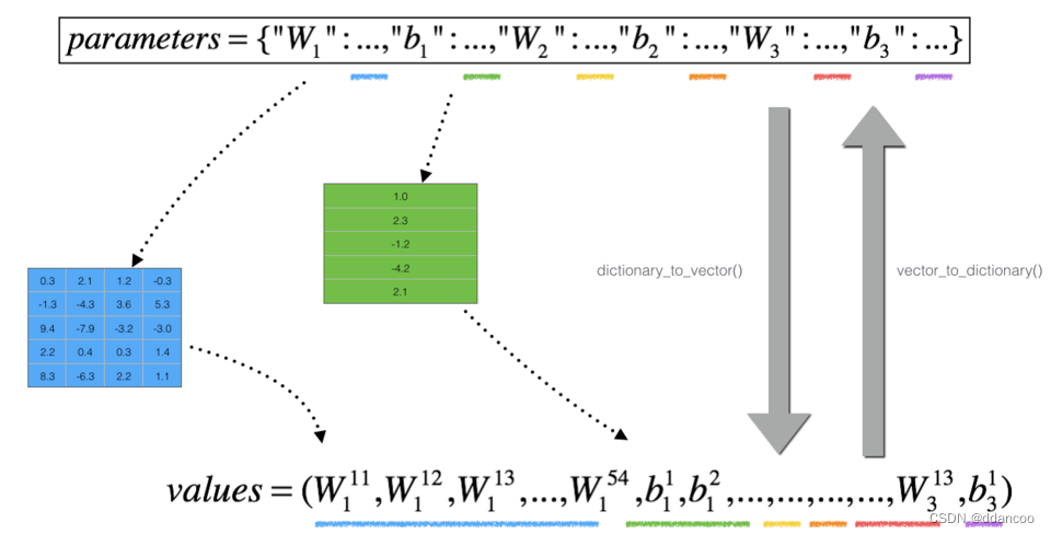
图2：dictionary_to_vector（）和vector_to_dictionary（）
你将在 gradient_check_n()中用到这些函数

我们还使用gradients_to_vector()将“gradients”字典转换为向量“grad”。

练习：实现gradient_check_n()。

说明：这是伪代码，可帮助你实现梯度检验。

For each i in num_parameters:

计算J_plus [i]：
将设为 `np.copy(parameters_values)`
1. 将 $\theta _{i}^{+}$ 设为 $\theta _{i}^{+}+\varepsilon$
2. 使用forward_propagation_n(x, y, vector_to_dictionary( $\theta ^{+}$ ))计算 $J_{i}^{+}$
计算J_minus [i]：也是用 $\theta ^{-}$
计算

因此，你将获得向量gradapprox，其中gradapprox[i]是相对于parameter_values[i]的梯度的近似值。现在，你可以将此gradapprox向量与反向传播中的梯度向量进行比较。就像一维情况（步骤1'，2'，3'）一样计算：

# GRADED FUNCTION: gradient_check_n

def gradient_check_n(parameters, gradients, X, Y, epsilon = 1e-7):
    """
    Checks if backward_propagation_n computes correctly the gradient of the cost output by forward_propagation_n
    
    Arguments:
    parameters -- python dictionary containing your parameters "W1", "b1", "W2", "b2", "W3", "b3":
    grad -- output of backward_propagation_n, contains gradients of the cost with respect to the parameters. 
    x -- input datapoint, of shape (input size, 1)
    y -- true "label"
    epsilon -- tiny shift to the input to compute approximated gradient with formula(1)
    
    Returns:
    difference -- difference (2) between the approximated gradient and the backward propagation gradient
    """
    
    # Set-up variables
    parameters_values, _ = dictionary_to_vector(parameters)
    
#将参数字典 parameters 转换为一个向量 parameters_values，并且返回转换后的向量和参数的维度信息（在这里用下划线 _ 表示不需要返回的变量）
#合成一个列数为1的列向量
#将参数字典中的所有参数值（比如权重矩阵和偏置向量）按照一定顺序连接成一个大的向量
    
    grad = gradients_to_vector(gradients)
    num_parameters = parameters_values.shape[0]
    J_plus = np.zeros((num_parameters, 1))
    J_minus = np.zeros((num_parameters, 1))
    gradapprox = np.zeros((num_parameters, 1))
    
    # Compute gradapprox
    for i in range(num_parameters):
        
        # Compute J_plus[i]. Inputs: "parameters_values, epsilon". Output = "J_plus[i]".
        # "_" is used because the function you have to outputs two parameters but we only care about the first one
        ### START CODE HERE ### (approx. 3 lines)
            # Step 1
        thetaplus = np.copy(parameters_values) 
#创建了一个名为 thetaplus 的变量，其中存储了参数向量 parameters_values 的副本
#通过创建副本，可以确保在修改 thetaplus 的同时不会影响到原始的 parameters_values。
            # Step 2
        thetaplus[i][0]=thetaplus[i][0]+epsilon
#theta[i][0]是 parameters_values 列向量中的第 i 个元素的值
        J_plus[i],_=forward_propagation_n(X,Y,vector_to_dictionary(thetaplus))

        ### END CODE HERE ###
        
        # Compute J_minus[i]. Inputs: "parameters_values, epsilon". Output = "J_minus[i]".
        ### START CODE HERE ### (approx. 3 lines)
            # Step 1
        thetaminus=np.copy(parameters_values)
            # Step 2  
        thetaminus[i][0]=thetaminus[i][0]-epsilon
        J_minus[i],_=forward_propagation_n(X,Y,vector_to_dictionary(thetaminus))
        ### END CODE HERE ###
        
        # Compute gradapprox[i]
        ### START CODE HERE ### (approx. 1 line)

        gradapprox[i]=(J_plus[i]-J_minus[i])/(2*epsilon)
        ### END CODE HERE ###
    
    # Compare gradapprox to backward propagation gradients by computing difference.
    ### START CODE HERE ### (approx. 1 line)
        # Step 1'
        numerator=np.linalg.norm(grad-gradapprox)
        # Step 2'
        denominator=np.linalg.norm(grad)+np.linalg.norm(gradapprox)
        # Step 3'
        difference=numerator/denominator
    ### END CODE HERE ###

    if difference > 1e-7:
        print ("\033[93m" + "There is a mistake in the backward propagation! difference = " + str(difference) + "\033[0m")
    else:
        print ("\033[92m" + "Your backward propagation works perfectly fine! difference = " + str(difference) + "\033[0m")
    
    return difference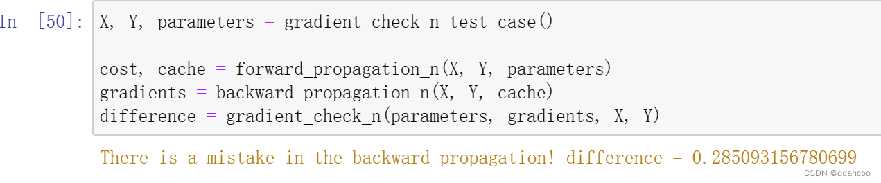

看起来backward_propagation_n代码似乎有错误！很好，你已经实现了梯度检验。返回到backward_propagation并尝试查找/更正错误（提示：检查dW2和db1）。如果你已解决问题，请重新运行梯度检验。请记住，如果修改代码，则需要重新执行定义backward_propagation_n()的单元格。

你可以进行梯度检验来证明你的导数计算的正确吗？即使作业的这一部分没有评分，我们也强烈建议你尝试查找错误并重新运行梯度检验，直到确信实现了正确的反向传播。

注意

梯度检验很慢！用逼近梯度在计算上是很耗费资源的。因此，我们不会在训练期间的每次迭代中都进行梯度检验。只需检查几次梯度是否正确。
至少如我们介绍的那样，梯度检验不适用于dropout。通常，你将运行不带dropout的梯度检验算法以确保你的backprop是正确的，然后添加dropout。

Nice！现在你可以确信你用于欺诈检测的深度学习模型可以正常工作！甚至可以用它来说服你的CEO。 :)

你在此笔记本中应记住的内容：

梯度检验可验证反向传播的梯度与梯度的数值近似值之间的接近度（使用正向传播进行计算）。
梯度检验很慢，因此我们不会在每次训练中都运行它。通常，你仅需确保其代码正确即可运行它，然后将其关闭并将backprop用于实际的学习过程。

ddancoo

关注

22
点赞
踩
26

收藏

觉得还不错? 一键收藏
0
评论
吴恩达深度学习L2W1作业3

欢迎来到本周的最后作业！在本作业中，你将学习实现和使用梯度检验。假设你是致力于在全球范围内提供移动支付的团队的一员，被上级要求建立深度学习模型来检测欺诈行为--每当有人进行支付时，你都应该确认该支付是否可能是欺诈性的，例如用户的帐户已被黑客入侵。但是模型的反向传播很难实现，有时还会有错误。因为这是关键的应用任务，所以你公司的CEO要反复确定反向传播的实现是正确的。CEO要求你证明你的反向传播实际上是有效的！为了保证这一点，你将应用到“梯度检验”。让我们开始做吧！
复制链接

扫一扫