


一、前置知识
1.1 tf.where
import tensorflow as tf
a = tf.constant([1,2,3,1,1])
b = tf.constant([0,1,3,4,5])
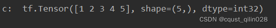
c = tf.where(tf.greater(a,b),a,b) #若a>b,返回a对应位置的元素,否则返回b对应位置的元素
print("c: ",c)
执行结果:
1.2 random.RandomState
生成0~1之间的随机数[0,1)
import tensorflow as tf
import numpy as np
rdm = np.random.RandomState(seed = 1) #seed = 常数表示每次生成随机数相同
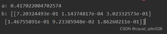
a = rdm.rand()#如果没有参数,那么返回标量
b = rdm.rand(2,3)
print("a:",a)
print("b:",b)
1.3 np.vstack
两个数组纵向上的叠加
import numpy as np

a = np.array([1,2,3])
b = np.array([4,5,6])
c = np.vstack((a,b))
print("c:\n",c)

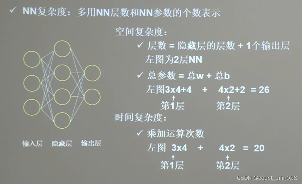
1.4 神经网络复杂度
只考虑参与计算的层的神经元
1.5 指数衰减学习率
先用较大的学习率,快速得到较优解,然后逐步减小学习率,使模型在训练后期稳定。
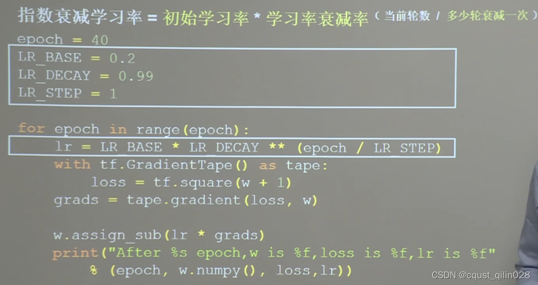
import  tensorflow as tf
w = tf.Variable(tf.constant(5,dtype=tf.float32))
a = 0.2 #学习率
epoch = 40 # 迭代次数
a_decay = 0.99
a_step = 1
#
for epoch in range(epoch):
    lr = a*a_decay**(epoch/a_step)
    with tf.GradientTape() as tape:
        loss = tf.square(w+1)
    grads = tape.gradient(loss,w) #.gradient函数告知loss对w求导
    w.assign_sub(lr*grads)
    print("After %s epoch,w is %f,loss is %f,learning rate is %f" %(epoch,w.numpy(),loss,lr))
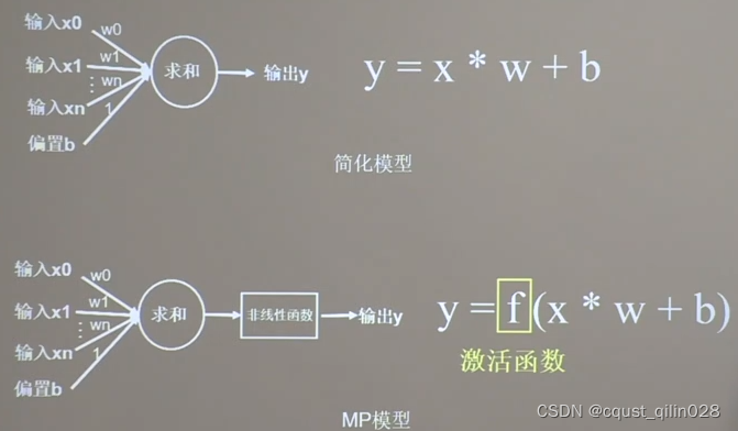
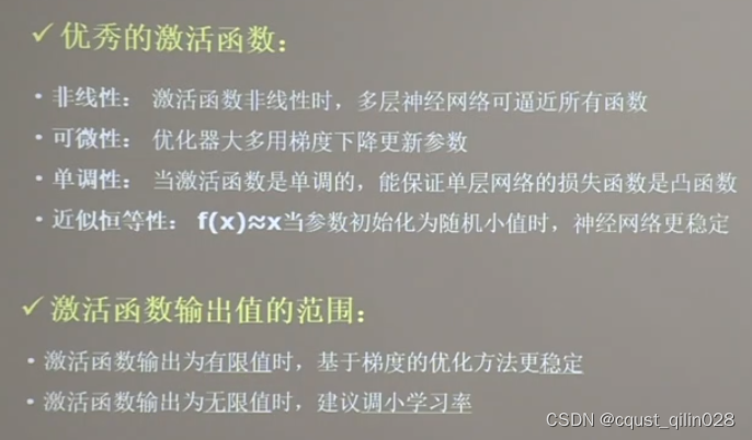
1.6 激活函数
1.6.1 Sigmoid函数
相当于对数据进行了归一化。
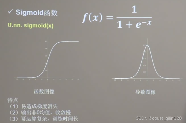
近年来用的较少,sigmoid函数的导数是0~0.25之间,而更新参数过程中需要链式求导,多次求导以后参数几乎为0,产生梯度消失,使得参数无法更新。
1.6.2 Tanh函数
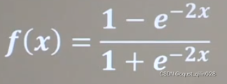
特点和sigmoid函数相同
1.6.3 Relu 函数
tf.nn.relu(x)
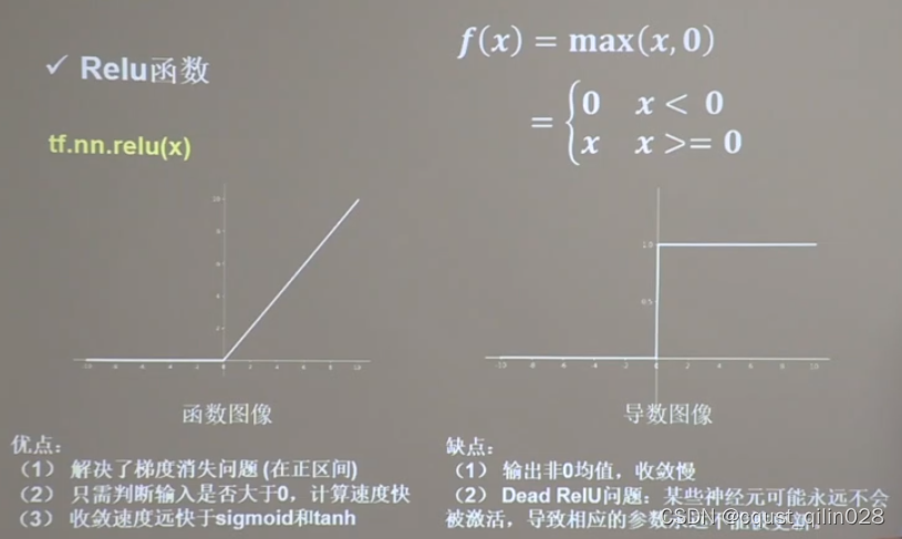
可以通过随机初始化,避免过多的负数特征进入激活函数,或者减小学习率
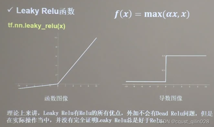
1.6.4 Leaky Relu
1.6.5 总结
二、损失函数(loss)
即预测值与已知答案(y_) 的差距
loss有三种估计方法:分别为:
- mse(Mean Squared Error)(均方误差)
- 自定义
- ce (Cross Entropy)(交叉熵)
y_:标准答案值 y:预测值
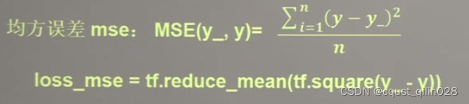
2.1 mse
mse的代码:
import tensorflow as tf
import numpy as np
SEED = 23455
rdm = np.random.RandomState(seed = SEED)
x = rdm.rand(32,2)
y_ = [[x1 + x2 + (rdm.rand()/10.0-0.05)] for(x1,x2) in x]
x = tf.cast(x,dtype=tf.float32)

w1 = tf.Variable(tf.random.normal([2,1],stddev=1,seed=1))
epoch = 15000
lr = 0.002

for epoch in range(epoch):
    with tf.GradientTape() as tape:
        y = tf.matmul(x,w1)
        loss_mse = tf.reduce_mean(tf.square(y_-y))

    grads = tape.gradient(loss_mse,w1)
    w1.assign_sub(lr*grads)

    if(epoch%500==0):
        print("After %d training steps,w1 is " % (epoch))
        print(w1.numpy(),"\n")
print("Final w1 is: ",w1.numpy())
2.2 自定义
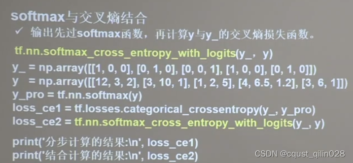
2.3 交叉熵(Cross Entropy)
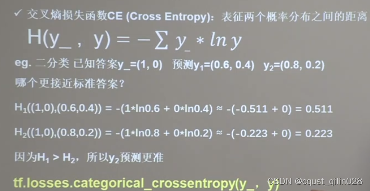
loss_ce1 = tf.losses.categorical_crossentropy([1,0],[0.6,0.4])
loss_ce2 = tf.losses.categorical_crossentropy([1,0],[0.8,0.2])
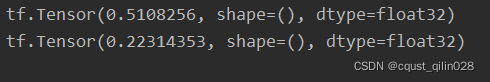
print(loss_ce1)
print(loss_ce2)
loss_ce2 等于 y_pro+loss_ce1
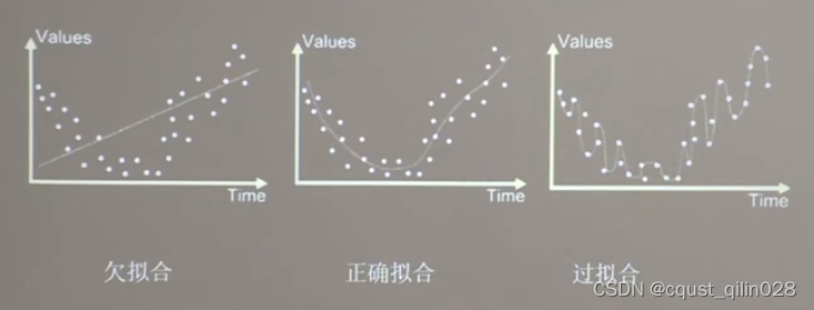
三、拟合
拟合分为欠拟合、正确拟合、过拟合
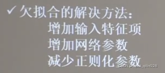
3.1 欠拟合的解决方法
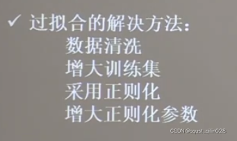
3.2 过拟合的解决方法
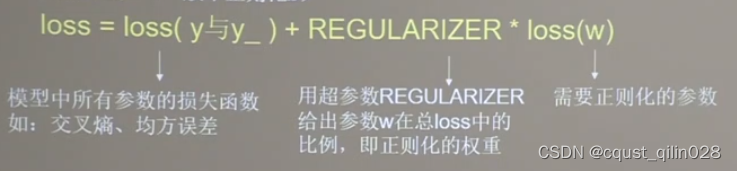
3.2.1 正则化缓解过拟合
正则化通常只对参数w使用,不对偏置b使用
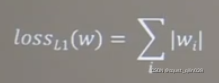
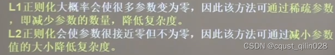
第一种正则化:(L1正则化)
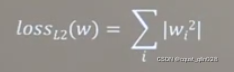
第二种正则化:
例子:通过中国大学mooc官网上该课程的class2文件中的dot.csv文件,配合课程代码,可以绘制如下图像:
import tensorflow as tf
from matplotlib import pyplot as plt
import numpy as np
import pandas as pd

df = pd.read_csv('F:\\dot.csv')
x_data = np.array(df[['x1','x2']])
y_data = np.array(df['y_c'])

x_train = np.vstack(x_data).reshape(-1,2)
y_train = np.vstack(y_data).reshape(-1,1)

Y_c = [['red' if y else 'blue'] for y in y_train]

# 矩阵相乘前必须强制转换
x_train = tf.cast(x_train,tf.float32)
y_train = tf.cast(y_train,tf.float32)

# 切分成若干个batch
train_db = tf.data.Dataset.from_tensor_slices((x_train,y_train)).batch(32)

# 需要训练的参数应使用tf.Variable()
# w1 b1 对应第一层
w1 = tf.Variable(tf.random.normal([2,11]),dtype=tf.float32)
b1 = tf.Variable(tf.constant(0.01,shape=[11]))

# w2 b2 对应第二层
w2 = tf.Variable(tf.random.normal([11,1]),dtype=tf.float32)
b2 = tf.Variable(tf.constant(0.01,shape=[1]))

lr = 0.005
epoch = 800

for epoch in range(epoch):
    for step,(x_train,y_train) in enumerate(train_db):
        with tf.GradientTape() as tape:
            h1 = tf.matmul(x_train,w1)+b1
            h1 = tf.nn.relu(h1)
            y = tf.matmul(h1,w2) + b2
            loss = tf.reduce_mean(tf.square(y_train-y))
        variables = [w1,b1,w2,b2]
        grads = tape.gradient(loss,variables)

        w1.assign_sub(lr*grads[0])
        b1.assign_sub(lr*grads[1])
        w2.assign_sub(lr*grads[2])
        b2.assign_sub(lr*grads[3])
    if epoch % 20 == 0:
        print('epoch: ',epoch,'loss:',float(loss))

# 预测部分
xx,yy = np.mgrid[-3:3:.1,-3:3:.1]
grid = np.c_[xx.ravel(),yy.ravel()]
grid = tf.cast(grid,tf.float32)

probs = []
for x_test in grid:
    h1 = tf.matmul([x_test],w1) + b1
    h1 = tf.nn.relu(h1)
    y = tf.matmul(h1,w2)+b2
    probs.append(y)

x1 = x_data[:,0]
x2 = x_data[:,1]

probs = np.array(probs).reshape(xx.shape)
plt.scatter(x1,x2,color=np.squeeze(Y_c))

plt.contour(xx,yy,probs,levels=[.5])
plt.show()
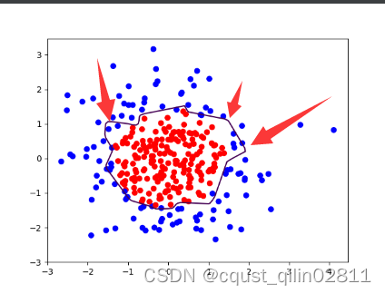
观察图像发现存在过拟合现象,尝试使用L2正则化缓解过拟合现象
优化后的代码:
import tensorflow as tf
from matplotlib import pyplot as plt
import numpy as np
import pandas as pd

df = pd.read_csv('F:\\dot.csv')# 绝对路径
x_data = np.array(df[['x1','x2']])
y_data = np.array(df['y_c'])

x_train = np.vstack(x_data).reshape(-1,2)
y_train = np.vstack(y_data).reshape(-1,1)

Y_c = [['red' if y else 'blue'] for y in y_train]

# 矩阵相乘前必须强制转换
x_train = tf.cast(x_train,tf.float32)
y_train = tf.cast(y_train,tf.float32)

# 切分成若干个batch
train_db = tf.data.Dataset.from_tensor_slices((x_train,y_train)).batch(32)

# 需要训练的参数应使用tf.Variable()
# w1 b1 对应第一层
w1 = tf.Variable(tf.random.normal([2,11]),dtype=tf.float32)
b1 = tf.Variable(tf.constant(0.01,shape=[11]))

# w2 b2 对应第二层
w2 = tf.Variable(tf.random.normal([11,1]),dtype=tf.float32)
b2 = tf.Variable(tf.constant(0.01,shape=[1]))

lr = 0.005
epoch = 800

for epoch in range(epoch):
    for step,(x_train,y_train) in enumerate(train_db):
        with tf.GradientTape() as tape:
            h1 = tf.matmul(x_train,w1)+b1
            h1 = tf.nn.relu(h1)
            y = tf.matmul(h1,w2) + b2
            loss_mse = tf.reduce_mean(tf.square(y_train-y))

            # 添加l2正则化
            loss_regularization = []
            loss_regularization.append(tf.nn.l2_loss(w1))
            loss_regularization.append(tf.nn.l2_loss(w2))
            loss_regularization = tf.reduce_sum(loss_regularization)
            loss = loss_mse + 0.03 * loss_regularization

        variables = [w1,b1,w2,b2]
        grads = tape.gradient(loss,variables)

        w1.assign_sub(lr*grads[0])
        b1.assign_sub(lr*grads[1])
        w2.assign_sub(lr*grads[2])
        b2.assign_sub(lr*grads[3])
    if epoch % 20 == 0:
        print('epoch: ',epoch,'loss:',float(loss))

# 预测部分
xx,yy = np.mgrid[-3:3:.1,-3:3:.1]
grid = np.c_[xx.ravel(),yy.ravel()]
grid = tf.cast(grid,tf.float32)

probs = []
for x_test in grid:
    h1 = tf.matmul([x_test],w1) + b1
    h1 = tf.nn.relu(h1)
    y = tf.matmul(h1,w2)+b2
    probs.append(y)

x1 = x_data[:,0]
x2 = x_data[:,1]

probs = np.array(probs).reshape(xx.shape)
plt.scatter(x1,x2,color=np.squeeze(Y_c))

plt.contour(xx,yy,probs,levels=[.5])
plt.show()
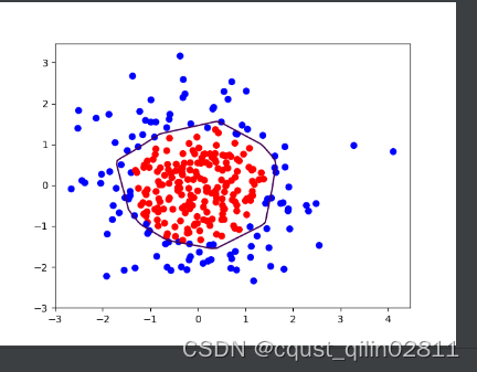
观察图片可以发现,采用正则化以后,曲线变得更加平缓,有效缓解了过拟合现象
四、神经网络参数优化器
就是梯度下降法之类的参数优化方法…
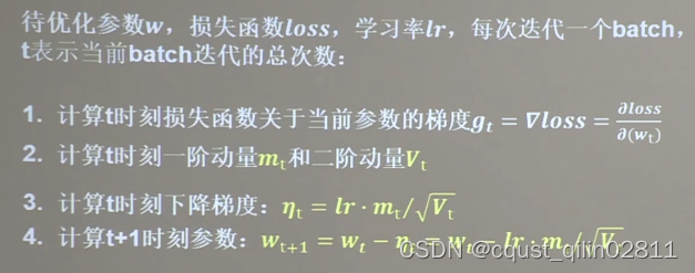
4.1 随机梯度下降法(SGD)
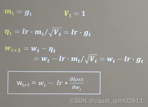
下一时刻的w等于当前时刻的w减去学习率乘以当前时刻的斜率


 370
370


 被折叠的 条评论
为什么被折叠?
被折叠的 条评论
为什么被折叠?
 到【灌水乐园】发言


