


吴恩达机器学习 第五周
0 总结
学习时间:2022.10.3~2022.10.9
- 完成练习二:逻辑回归及逻辑回归的正则化代码编写
- 学习神经网络的假设函数和前向传播的表示
- 学习如何使用神经网络解决多分类问题
- 完成练习三:逻辑回归多分类部分
1 练习二:逻辑回归
1.1 逻辑回归
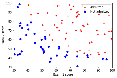
==背景:==假设你是一个大学系的管理员,你需要根据每个申请人的两次考试的结果决定录取机会。
1.1.1 可视化数据
任务:完成plotData.py,画出figure1,横轴和纵轴是两个考试分数,正和负样本用不同符号表示。
代码:参考链接: python绘制散点图
def plot_data(X, y):
    plt.figure()

    # ===================== Your Code Here =====================
    # Instructions : Plot the positive and negative examples on a
    #                2D plot, using the marker="+" for the positive
    #                examples and marker="o" for the negative examples
    #
    # 分离正负样本
    positive = X[y==1]
    negative = X[y==0]

    plt.scatter(positive[:,0],positive[:,1],marker='+',c='red',label='Admitted') #画出正样本
    plt.scatter(negative[:,0],negative[:,1],marker='o',c='blue',label='Not Admitted') #画出正样本
结果
1.1.2 sigmoid函数
tips:np.r_是按列连接两个矩阵,就是把两矩阵上下相加,要求列数相等。
np.c_是按行连接两个矩阵,就是把两矩阵左右相加,要求行数相等。
sigmoid函数:
g
(
z
)
=
1
1
+
e
−
z
g(z)=\frac{1}{1+e^{-z}}
g(z)=1+e−z1
任务:完成sigmoid函数
代码:
def sigmoid(z):
    # 初始化
    g = np.zeros(z.size)

    # ===================== Your Code Here =====================
    # Instructions : Compute the sigmoid of each value of z (z can be a matrix,
    #                vector or scalar
    #
    # Hint : Do not import math
    g = 1/(1+np.exp(-z))

    return g
1.1.3 代价函数和梯度
tips:
h
θ
(
x
)
=
1
1
+
e
−
θ
T
x
h_\theta(x)=\frac{1}{1+e^{-\theta^Tx}}
hθ(x)=1+e−θTx1
J
(
θ
)
=
1
m
∑
i
=
1
m
C
o
s
t
(
h
θ
(
x
(
i
)
)
,
y
(
i
)
)
J(\theta)=\frac{1}{m}\sum_{i=1}^mCost(h_\theta(x^{(i)}),y^{(i)})
J(θ)=m1i=1∑mCost(hθ(x(i)),y(i))其中:
C
o
s
t
(
h
θ
(
x
)
,
y
)
=
−
y
l
o
g
(
h
θ
(
x
)
)
−
(
1
−
y
)
l
o
g
(
1
−
h
θ
(
x
)
)
Cost(h_\theta(x),y)=-ylog(h_\theta(x))-(1-y)log(1-h_\theta(x))
Cost(hθ(x),y)=−ylog(hθ(x))−(1−y)log(1−hθ(x))注意:
y
=
0
y=0
y=0或者
y
=
1
y=1
y=1。
所以,代价函数:
J
(
θ
)
=
1
m
∑
i
=
1
m
C
o
s
t
(
h
θ
(
x
(
i
)
)
,
y
(
i
)
)
=
−
1
m
[
∑
i
=
1
m
y
(
i
)
l
o
g
(
h
θ
(
x
(
i
)
)
)
+
(
1
−
y
(
i
)
)
l
o
g
(
1
−
h
θ
(
x
(
i
)
)
)
]
\begin{align} J(\theta) & = \frac{1}{m}\sum_{i=1}^mCost(h_\theta(x^{(i)}),y^{(i)}) \notag\\ & = -\frac{1}{m}[\sum_{i=1}^m y^{(i)} log(h_\theta(x^{(i)}))+(1-y^{(i)} )log(1-h_\theta(x^{(i)} ))]\notag \end{align}
J(θ)=m1i=1∑mCost(hθ(x(i)),y(i))=−m1[i=1∑my(i)log(hθ(x(i)))+(1−y(i))log(1−hθ(x(i)))]当前要做的是:寻找合适的参数
θ
\theta
θ使得
J
(
θ
)
J(\theta)
J(θ)最小;找到
θ
\theta
θ后,在给定某个输入
x
x
x可以预测出
h
θ
(
x
)
h_\theta(x)
hθ(x)。
作法:
Repeat{
θ
j
:
=
θ
j
−
α
∂
J
(
θ
)
∂
θ
j
:
=
θ
j
−
α
∑
i
=
1
m
(
h
θ
(
x
(
i
)
)
−
y
(
i
)
)
x
j
(
i
)
\begin{align} \theta_j& :=\theta_j-\alpha\frac{\partial J(\theta)}{\partial \theta_j} \notag\\ & :=\theta_j-\alpha\sum_{i=1}^m(h_\theta(x^{(i)})-y^{(i)})x_j^{(i)}\notag \end{align}
θj:=θj−α∂θj∂J(θ):=θj−αi=1∑m(hθ(x(i))−y(i))xj(i)}
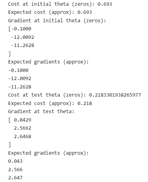
任务:完成costFunction.py
注意:如果dot的两个参数是向量,则只要求他们的维度相等就可以直接dot。
代码:
def cost_function(theta, X, y):
    m = y.size

    # You need to return the following values correctly
    cost = 0
    # n+1
    grad = np.zeros(theta.shape)

    # ===================== Your Code Here =====================
    # Instructions : Compute the cost of a particular choice of theta
    #                You should set cost and grad correctly.
    #
    # 计算cost和grad
    # 假设函数h是m维向量
    h = sigmoid(np.dot(X,theta))
    #
    term1 = -np.dot(y,np.log(h))
    term2 = -np.dot(1-y,np.log(1-h))
    cost = (term1 + term2)/m
    grad = np.dot(h-y,X)/m


    # ===========================================================

    return cost, grad
运行结果:
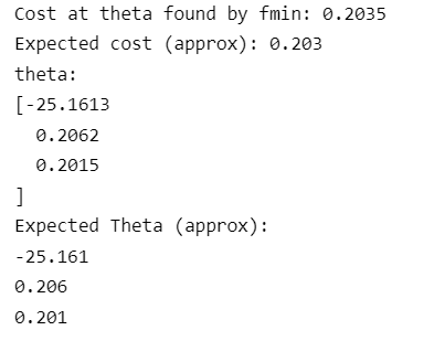
1.1.3 fmin_bfgs优化函数
代码:
'''
    fmin_bfgs优化函数
    第一个参数是计算代价的函数
    第二个参数是计算梯度的函数
    参数x0传入初始化的theta值
    maxiter设置最大迭代优化次数
'''
theta, cost, *unused = opt.fmin_bfgs(f=cost_func, fprime=grad_func, x0=initial_theta, maxiter=400, full_output=True, disp=False)
运行结果:
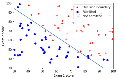
1.1.4 评估逻辑回归
任务:完成predict.py,输入48和45,会得到录取概率为0.776。
代码:
def predict(theta, X):
    m = X.shape[0]

    # Return the following variable correctly
    p = np.zeros(m)

    # ===================== Your Code Here =====================
    # Instructions : Complete the following code to make predictions using
    #                your learned logistic regression parameters.
    #                You should set p to a 1D-array of 0's and 1's
    #
    p = sigmoid(X.dot(theta))
    p[p>=0.5] = 1
    p[p<0.5] = 0

    # ===========================================================

    return p
1.2 正则化的逻辑回归
1.2.1 数据可视化

数据没有被直线分割成正和负两部分,因此线性的逻辑回归并不能很好地分割这部分数据集。
1.2.2 特征映射(!重要)
一个更好地拟合数据的方法是创造更多的特征。在mapFeauture.py中,我们将两个特征映射成x1、x2的六次方的特征多项式。

这样我们就将两个特征变成28位的向量。在这组高纬度的特征向量训练出来的逻辑回归分类器,将有更复杂的决策边界和非线性。但是,也可能会出现过拟合问题,因此我们需要对逻辑回归进行正则化。
1.2.3 代价函数的梯度
任务:完成costFunctionReg.py
注意:python下标从0开始,如图所示:

代码:
def cost_function_reg(theta, X, y, lmd):
    m = y.size

    # You need to return the following values correctly
    cost = 0
    grad = np.zeros(theta.shape)

    # ===================== Your Code Here =====================
    # Instructions : Compute the cost of a particular choice of theta
    #                You should set cost and grad correctly.
    #
    # h:(m,1)
    h = sigmoid(X.dot(theta))
    m1 = -y.dot(np.log(h))
    m2 = -(1-y).dot(np.log(1-h))
    m3 = theta[1:].dot(theta[1:])
    cost = (m1+m2)/m + lmd*m3/(2*m)

    grad = X.T.dot(h-y)/m
    grad[1:] += theta[1:]*lmd/m

    # ===========================================================

    return cost, grad
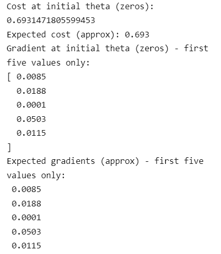
运行结果:
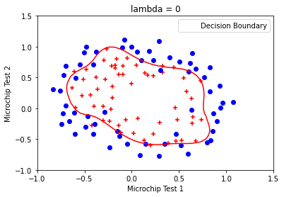
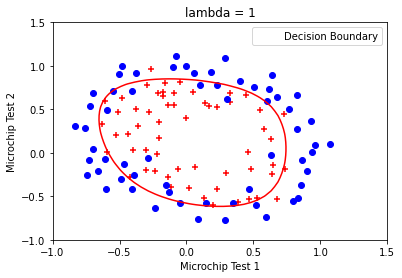
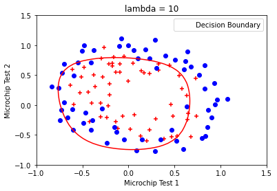
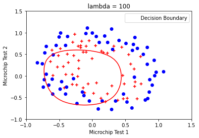
1.2.4 决策边界
任务:使用fmin_bfgs训练参数
θ
\theta
θ,并绘制决策边界。使用不同的KaTeX parse error: Undefined control sequence: \ambda at position 1: \̲a̲m̲b̲d̲a̲,观察决策边界的变化。
结果:
2 神经网络的表示
2.1 神经网络假设函数
逻辑单元

输入为 x 0 , x 1 , x 2 , x 3 x_0,x_1,x_2,x_3 x0,x1,x2,x3, x 0 x_0 x0为偏差单元,有时候不写,永远为1。
激励函数为sigmoid函数。
假设函数为 h θ ( x ) = 1 1 + e − z h_\theta(x)=\frac{1}{1+e^{-z}} hθ(x)=1+e−z1
权重为θ \theta θ
神经网络


Layer1:输入层,Layer2:隐藏层(可不止一层),Layer3:输出层。
a i j a_i^j aij:第 j j j层的第 i i i个激活项。(上角标表示层数)
Θ j \Theta^j Θj:第 j j j层到第 j + 1 j+1 j+1层的权重。
如果神经网络在第 j j j层有 s j s_j sj个单元,在第 j + 1 j+1 j+1层有 s j + 1 s_{j+1} sj+1个单元,那么 Θ j = s j + 1 × ( s j + 1 ) \Theta_j=s_{j+1}\times(s_j+1) Θj=sj+1×(sj+1)(不包含1),比如这里, Θ 1 ∈ R 3 × 4 \Theta_1\in\mathbb{R}^{3\times4} Θ1∈R3×4
2.2 前向传播
如图,假设输入:
x
=
a
(
1
)
=
[
x
0
x
1
x
2
x
3
]
∈
R
4
x=a^{(1)}=\begin{bmatrix} x_0 \\ x_1 \\ x_2 \\ x_3 \end{bmatrix}\in\mathbb{R}^4
x=a(1)=⎣
⎡x0x1x2x3⎦
⎤∈R4,其中
x
0
=
1
x_0 = 1
x0=1。那么,定义:
z
(
2
)
=
[
z
1
(
2
)
z
2
(
2
)
z
3
(
2
)
]
=
[
Θ
10
(
1
)
x
0
+
Θ
11
(
1
)
x
1
+
Θ
12
(
1
)
x
2
+
Θ
13
(
1
)
x
3
Θ
20
(
1
)
x
0
+
Θ
21
(
1
)
x
1
+
Θ
22
(
1
)
x
2
+
Θ
23
(
1
)
x
3
Θ
30
(
1
)
x
0
+
Θ
31
(
1
)
x
1
+
Θ
32
(
1
)
x
2
+
Θ
33
(
1
)
x
3
]
=
Θ
(
1
)
a
(
1
)
∈
R
3
z^{(2)}=\begin{bmatrix} z^{(2)}_1 \\ z^{(2)}_2 \\ z^{(2)}_3 \end{bmatrix} = \begin{bmatrix} \Theta^{(1)}_{10}x_0+\Theta^{(1)}_{11}x_1+\Theta^{(1)}_{12}x_2+\Theta^{(1)}_{13}x_3\\ \Theta^{(1)}_{20}x_0+\Theta^{(1)}_{21}x_1+\Theta^{(1)}_{22}x_2+\Theta^{(1)}_{23}x_3\\ \Theta^{(1)}_{30}x_0+\Theta^{(1)}_{31}x_1+\Theta^{(1)}_{32}x_2+\Theta^{(1)}_{33}x_3 \end{bmatrix} = \Theta^{(1)}a^{(1)} \in\mathbb{R}^3
z(2)=⎣
⎡z1(2)z2(2)z3(2)⎦
⎤=⎣
⎡Θ10(1)x0+Θ11(1)x1+Θ12(1)x2+Θ13(1)x3Θ20(1)x0+Θ21(1)x1+Θ22(1)x2+Θ23(1)x3Θ30(1)x0+Θ31(1)x1+Θ32(1)x2+Θ33(1)x3⎦
⎤=Θ(1)a(1)∈R3,理解到矩阵中每一行是该层某个神经元的计算公式。那么:
a
(
2
)
=
g
(
z
(
2
)
)
∈
R
3
a^{(2)}=g(z^{(2)})\in\mathbb{R}^3
a(2)=g(z(2))∈R3,其中,
g
g
g为sigmoid函数。至此,第二层三个神经元的值计算出来了。
将
a
0
(
2
)
=
1
a^{(2)}_0=1
a0(2)=1加入到矩阵
a
(
2
)
a^{(2)}
a(2)中,
a
(
2
)
a^{(2)}
a(2)变为四维向量。
重复上述步骤:
z
(
3
)
=
Θ
(
2
)
a
(
2
)
,
z^{(3)}=\Theta^{(2)}a^{(2)},
z(3)=Θ(2)a(2),
h
Θ
(
x
)
=
a
(
3
)
=
g
(
z
(
3
)
)
h_\Theta(x)=a^{(3)}=g(z^{(3)})
hΘ(x)=a(3)=g(z(3))。
2.3 神经网络应用举例
逻辑与

可以看到,当
Θ
=
[
−
30
20
20
]
\Theta=\begin{bmatrix} -30 \\ 20 \\ 20 \end{bmatrix}
Θ=⎣
⎡−302020⎦
⎤的时候,这个神经网络可以模拟逻辑与。
逻辑或

可以看到,当
Θ
=
[
−
10
20
20
]
\Theta=\begin{bmatrix} -10 \\ 20 \\ 20 \end{bmatrix}
Θ=⎣
⎡−102020⎦
⎤的时候,这个神经网络可以模拟逻辑或。
2.4 同或门
利用之前设计的神经网络设计一个同或门。
(!看清楚颜色对应)

2.5 多分类问题

3 练习三:多分类问题和神经网络
3.1 多分类问题
data = scio.loadmat('ex3data1.mat')
X = data['X']
y = data['y'].flatten()
ex3data1.mat中数据:
一共有5000个样本,每个样本是20x20像素的图像。每个像素使用浮点数表示灰度。y是1-10的数字。现在需要使用逻辑回归和神经网络识别手写数字0~9。

3.1.1 数据可视化

随机抽取的100个样本示例。
3.1.2 逻辑回归向量化
代价函数
在没有正则化的逻辑回归中,代价函数的表达式:

因此我们需要先计算
h
θ
(
x
(
i
)
)
h_\theta(x^{(i)})
hθ(x(i)),假设函数表达式如下:

因此我们定义:

m m m:样本个数。
x ( i ) x^{(i)} x(i):第 i i i个样本的n+1个数据,是列向量。
则有:

如果 a a a和 b b b是向量,则 a T b a^Tb aTb= b T a b^Ta bTa
梯度
在没有正则化的逻辑回归中,梯度的表达式:

将每一步的偏导写出:

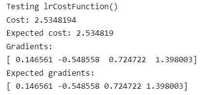
任务:完成lrCostFunctio.py
代码:(正则化)
def compute_cost(theta,X,y,lmd):
    cost = 0
    m = y.size
    h = sigmoid(X.dot(theta))

    temp1 = -np.dot(y.T,np.log(h))
    temp2 = -np.dot((1-y).T,np.log(1-h))
    temp3 = np.dot(theta[1:].T,theta[1:])
    cost = (temp1+temp2)/m+temp3*lmd/(2*m)

    return cost

def compute_grad(theta,X,y,lmd):
    m = y.size
    grad = np.zeros(theta.shape)

    h = sigmoid(X.dot(theta))
    temp4 = h-y
    grad = np.dot(X.T, temp4)/m
    grad[1:] += theta[1:]*lmd/m

    return grad

def lr_cost_function(theta, X, y, lmd):

    cost = compute_cost(theta, X, y, lmd)
    grad = compute_grad(theta, X, y, lmd)

    return cost, grad
运行结果:
3.1.3 多分类问题
在多分类问题中,参数矩阵
Θ
∈
R
K
×
(
N
+
1
)
\Theta \in \mathbb{R}^{K\times(N+1)}
Θ∈RK×(N+1),K为分类的类别个数,也就是说,每一行表示了每一类的参数。在手写识别问题中,
K
=
10
K=10
K=10,注意到
y
=
10
y=10
y=10的时候,表示手写图片是0。
任务:完成oneVsAll.py
代码:
def one_vs_all(X, y, num_labels, lmd):
    # Some useful variables
    (m, n) = X.shape

    # You need to return the following variables correctly
    all_theta = np.zeros((num_labels, n + 1))
    initial_theta = np.zeros(n+1)

    # Add ones to the X data 2D-array
    X = np.c_[np.ones(m), X]

    # 循环:每一类进行一次循环
    # i = 0,1,2,...num_labels-1
    for i in range(num_labels):
        print('Optimizing for handwritten number {}...'.format(i))
        # ===================== Your Code Here =====================
        # Instructions : You should complete the following code to train num_labels
        #                logistic regression classifiers with regularization
        #                parameter lambda
        #
        #
        # Hint: you can use y == c to obtain a vector of True(1)'s and False(0)'s that tell you
        #       whether the ground truth is true/false for this class
        #
        # Note: For this assignment, we recommend using opt.fmin_cg to optimize the cost
        #       function. It is okay to use a for-loop (for c in range(num_labels) to
        #       loop over the different classes
        #


        # 手写数字0的时候y=10
        iclass = i if i  else 10
        y_temp = np.array([1 if iy == iclass else 0 for iy in y ])
        ''' fmin_cg优化函数 第一个参数是计算代价的函数 第二个参数是计算梯度的函数 参数x0传入初始化的theta值
            args传入训练样本的输入特征矩阵X,对应的2分类新标签y,正则化惩罚项系数lmd
            maxiter设置最大迭代优化次数
        '''
        res = opt.fmin_cg(lCF.compute_cost,fprime = lCF.compute_grad,x0 = initial_theta,\
                                    args=(X,y_temp,lmd),maxiter=50,disp=False,full_output=True)
        all_theta[i] = res[0]
        # ============================================================
        print('Done')

    return all_theta
3.1.4 多分类预测
任务:完成predictOneVsAll.py
tips: argmax的用法
代码:
def predict_one_vs_all(all_theta, X):
    m = X.shape[0]
    num_labels = all_theta.shape[0]

    # You need to return the following variable correctly;
    p = np.zeros(m)

    # Add ones to the X data matrix
    X = np.c_[np.ones(m), X]

    # ===================== Your Code Here =====================
    # Instructions : Complete the following code to make predictions using
    #                your learned logistic regression parameters (one vs all).
    #                You should set p to a vector of predictions (from 1 to
    #                num_labels)
    #
    # Hint : This code can be done all vectorized using the max function
    #        In particular, the max function can also return the index of the
    #        max element, for more information see 'np.argmax' function.
    #

    poss = sigmoid(X.dot(all_theta.T))
    # 每一行最大值的下标
    index_max = np.argmax(poss,axis = 1)
    p = np.array([index if index else 10 for index in index_max])

    return p
运行结果:


 605
605


 被折叠的 条评论
为什么被折叠?
被折叠的 条评论
为什么被折叠?
 到【灌水乐园】发言


