吴恩达ML WEEK8+9 练习四：神经网络+SVM+聚类

---

0 总结

学习时间：2022.10.24~2022.11.6

• 编写练习四神经网络的前向反馈和后向传播代码。
• 学习支持向量机SVM。
• 学习聚类算法（K均值算法）。

---

–

1 练习四：神经网络

ex4.m - 指导你在整个练习。
ex4data1.mat - 手写数字的训练集。
ex4weights.mat -练习4的神经网络参数。
submit.m - Submission script that sends your solutions to our servers
displayData.m - 数据可视化。
fmincg.m - 最小化程序函数。
sigmoid.m - Sigmoid函数。
computeNumericalGradient.m - 数值上的梯度计算。
checkNNGradients.m - 梯度检查函数。
debugInitializeWeights.m - 权重初始化函数。
predict.m - 神经网络预测函数。
[?] sigmoidGradient.m - 计算sigmoid函数的梯度。
[?] randInitializeWeights.m - 随机初始化权重。
[?] nnCostFunction.m - 神经网络代价函数。

---

1.1 神经网络

任务：
使用反向传播算法更新神经网络的参数。

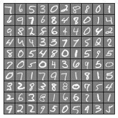
1.1.1 数据可视化

一共有5000个训练样本，，每个训练样本是20像素x20像素（灰度）的图像。这20x20的像素被伸展成一个400维的向量，存放在矩阵X中（每一行表示一个样本）。
结果：

1.1.2 模型表述

输入层有400个单元，隐藏层有25个单元，输出层有10个单元。
ex4weights.mat中是已经训练好了的${\Theta }^{(1)},{\Theta }^{(2)}$的值，${\Theta }^{(1)}$是 25 x 401
的矩阵，${\Theta }^{(2)}$是10 x 26的矩阵。

1.1.3 前向和代价函数

任务：完成nnCostFunction.py的代码。
tips：代价函数表达式（本代码不含正则化）：

要注意，正则项也是不包括$i=0$的！

y:（0表示第1个类别，1表示第2个类别，以此类推）

如何将X添加一列全为1
代码：

import numpy as np
from sigmoid import *

def expend_y(y,num_labels):
    # 每个y展开成长度为10的向量
    result = []
    for i in y:
        y_array = np.zeros(num_labels)
        y_array[i-1]=1
        result.append(y_array)

    return np.array(result)

# 前向传播算法以计算假设h
# m:样本个数
def ForwardPropagation(X,theta1,theta2,m):
    # 第一层神经元的值
    a_1 = np.c_[np.ones(m),X]
    # 第二层神经元的值
    a_2 = sigmoid(np.dot(a_1,theta1.T))
    # 第三层神经元的值
    a_2 = np.c_[np.ones(m),a_2]
    a_3 = sigmoid(np.dot(a_2,theta2.T))# (m,10)

    return a_3

def CostFunction(X,y,theta1,theta2,m,num_labels):
    # 1.首先将y转换，比如y[0]=6，那么转换后y[0]=[0 0 0 0 0 0 1 0 0 0]
    y_temp = expend_y(y, num_labels) # (m,10)
    h= ForwardPropagation(X,theta1,theta2,m) # (m,10)
    cost = 0

    term1 = -y_temp*np.log(h) # (m,k)
    term2 = -(1-y_temp)*np.log(1-h) # (m,k)
    cost = np.sum(term1+term2)/m

    return cost   

def nn_cost_function(nn_params, input_layer_size, hidden_layer_size, num_labels, X, y, lmd):
    # Reshape nn_params back into the parameters theta1 and theta2, the weight 2-D arrays
    # for our two layer neural network
    theta1 = nn_params[:hidden_layer_size * (input_layer_size + 1)].reshape(hidden_layer_size, input_layer_size + 1)
    theta2 = nn_params[hidden_layer_size * (input_layer_size + 1):].reshape(num_labels, hidden_layer_size + 1)

    # Useful value
    m = y.size

    # You need to return the following variables correctly
    cost = 0
    theta1_grad = np.zeros(theta1.shape)  # 25 x 401
    theta2_grad = np.zeros(theta2.shape)  # 10 x 26

    # ===================== Your Code Here =====================
    # Instructions : You should complete the code by working thru the
    #                following parts
    #
    # Part 1 : Feedforward the neural network and return the cost in the
    #          variable cost. After implementing Part 1, you can verify that your
    #          cost function computation is correct by running ex4.py
    #          前向回归返回cost
    #
    # Part 2: Implement the backpropagation algorithm to compute the gradients
    #         theta1_grad and theta2_grad. You should return the partial derivatives of
    #         the cost function with respect to theta1 and theta2 in theta1_grad and
    #         theta2_grad, respectively. After implementing Part 2, you can check
    #         that your implementation is correct by running checkNNGradients
    #         使用反向传播计算梯度theta1_grad and theta2_grad并返回
    #
    #         Note: The vector y passed into the function is a vector of labels
    #               containing values from 1..K. You need to map this vector into a 
    #               binary vector of 1's and 0's to be used with the neural network
    #               cost function.
    #               y是从1到k的数
    #
    #         Hint: We recommend implementing backpropagation using a for-loop
    #               over the training examples if you are implementing it for the 
    #               first time.
    #
    # Part 3: Implement regularization with the cost function and gradients.
    #
    #         Hint: You can implement this around the code for
    #               backpropagation. That is, you can compute the gradients for
    #               the regularization separately and then add them to theta1_grad
    #               and theta2_grad from Part 2.
    #
    cost = CostFunction(X,y,theta1,theta2,m,num_labels)
    # ====================================================================================
    # Unroll gradients
    grad = np.concatenate([theta1_grad.flatten(), theta2_grad.flatten()])

    return cost, grad

运行结果：

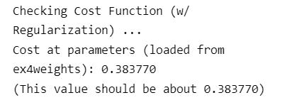
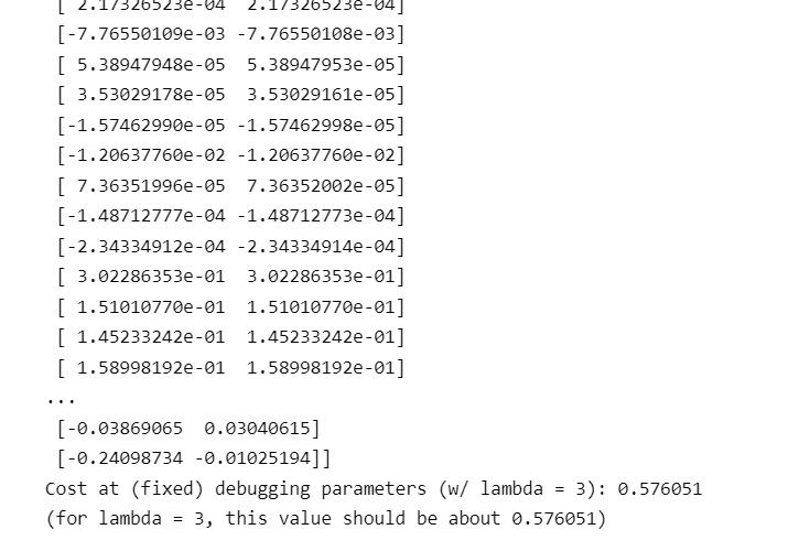
1.1.4 代价函数正则化

任务：
补充nnCostFunction.py中代价函数的正则项。
代码：

import numpy as np
from sigmoid import *

def expend_y(y,num_labels):
    # 每个y展开成长度为10的向量
    result = []
    for i in y:
        y_array = np.zeros(num_labels)
        y_array[i-1]=1
        result.append(y_array)

    return np.array(result)

# 前向传播算法以计算假设h
# m:样本个数
def ForwardPropagation(X,theta1,theta2,m):
    # 第一层神经元的值
    a_1 = np.c_[np.ones(m),X]
    # 第二层神经元的值
    a_2 = sigmoid(np.dot(a_1,theta1.T))
    # 第三层神经元的值
    a_2 = np.c_[np.ones(m),a_2]
    a_3 = sigmoid(np.dot(a_2,theta2.T))# (m,10)

    return a_3

def CostFunction(X,y,theta1,theta2,m,num_labels,lmd):
    # 1.首先将y转换，比如y[0]=6，那么转换后y[0]=[0 0 0 0 0 0 1 0 0 0]
    y_temp = expend_y(y, num_labels) # (m,10)
    h= ForwardPropagation(X,theta1,theta2,m) # (m,10)
    cost = 0

    term1 = -y_temp*np.log(h) # (m,k)
    term2 = -(1-y_temp)*np.log(1-h) # (m,k)
    reg = lmd*(np.sum(theta1[:,1:]**2)+np.sum(theta2[:,1:]**2))/(2*m)
    cost = np.sum(term1+term2)/m + reg

    return cost   

def nn_cost_function(nn_params, input_layer_size, hidden_layer_size, num_labels, X, y, lmd):
    # Reshape nn_params back into the parameters theta1 and theta2, the weight 2-D arrays
    # for our two layer neural network
    theta1 = nn_params[:hidden_layer_size * (input_layer_size + 1)].reshape(hidden_layer_size, input_layer_size + 1)
    theta2 = nn_params[hidden_layer_size * (input_layer_size + 1):].reshape(num_labels, hidden_layer_size + 1)

    # Useful value
    m = y.size

    # You need to return the following variables correctly
    cost = 0
    theta1_grad = np.zeros(theta1.shape)  # 25 x 401
    theta2_grad = np.zeros(theta2.shape)  # 10 x 26

    # ===================== Your Code Here =====================
    # Instructions : You should complete the code by working thru the
    #                following parts
    #
    # Part 1 : Feedforward the neural network and return the cost in the
    #          variable cost. After implementing Part 1, you can verify that your
    #          cost function computation is correct by running ex4.py
    #          前向回归返回cost
    #
    # Part 2: Implement the backpropagation algorithm to compute the gradients
    #         theta1_grad and theta2_grad. You should return the partial derivatives of
    #         the cost function with respect to theta1 and theta2 in theta1_grad and
    #         theta2_grad, respectively. After implementing Part 2, you can check
    #         that your implementation is correct by running checkNNGradients
    #         使用反向传播计算梯度theta1_grad and theta2_grad并返回
    #
    #         Note: The vector y passed into the function is a vector of labels
    #               containing values from 1..K. You need to map this vector into a 
    #               binary vector of 1's and 0's to be used with the neural network
    #               cost function.
    #               y是从1到k的数
    #
    #         Hint: We recommend implementing backpropagation using a for-loop
    #               over the training examples if you are implementing it for the 
    #               first time.
    #
    # Part 3: Implement regularization with the cost function and gradients.
    #
    #         Hint: You can implement this around the code for
    #               backpropagation. That is, you can compute the gradients for
    #               the regularization separately and then add them to theta1_grad
    #               and theta2_grad from Part 2.
    #
    cost = CostFunction(X,y,theta1,theta2,m,num_labels,lmd)






    # ====================================================================================
    # Unroll gradients
    grad = np.concatenate([theta1_grad.flatten(), theta2_grad.flatten()])

    return cost, grad

结果：

---

1.2 反向传播

完成对代价函数的反向传播以获得梯度。

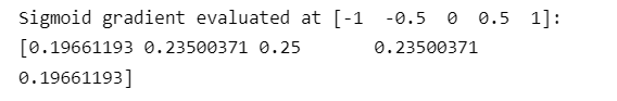
1.2.1 sigmoid函数的梯度

当z是一个很大的值时（无论正还是负），sigmoid函数的梯度都是0；当z等于0时，sigmoid的梯度是0.25。
任务：完成sigmoidGradient.py函数
代码：

import numpy as np
from sigmoid import *


def sigmoid_gradient(z):
    g = np.zeros(z.shape)

    # ===================== Your Code Here =====================
    # Instructions : Compute the gradient of the sigmoid function evaluated at
    #                each value of z (z can be a matrix, vector or scalar)
    #
    g=sigmoid(z)*(1-sigmoid(z))

    # ===========================================================

    return g

运行结果：

1.2.2 随机初始化

任务：randInitializeWeights.py
tips：

np.random.uniform介绍
代码：

import numpy as np


def rand_initialization(l_in, l_out):
    # You need to return the following variable correctly

    # ===================== Your Code Here =====================
    # Instructions : Initialize w randomly so that we break the symmetry while
    #                training the neural network
    #
    # Note : The first column of w corresponds to the parameters for the bias unit
    #
    epsilon = 0.12

    w = np.random.uniform(-epsilon, epsilon, (l_out, 1 + l_in))

    # ===========================================================

    return w

1.2.3 反向传播

tips：

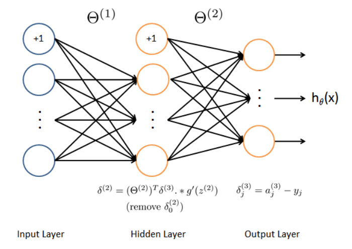
首先对于每一个训练样本，我们使用前向传播计算出每个激活分子（包括假设函数）。然后在每一层的节点，我们计算出“误差项”，衡量节点对我们输出误差的影响。

任务：完成nncostfunction.py的反向传播部分
代码：

# 计算梯度（包含正则化）
# X:(m,401)
# y_temp:(m,10)
# theta1:(25,401)
# theta2:(10,26)

def computeGrad(X,y_temp,theta1,theta2,lmd,m):
    a_1,z_2,a_2,z_3,a_3= ForwardPropagation(X,theta1,theta2,m) # (m,10)
    # 第三层
    delta_3 = a_3-y_temp #(m,10)
    
    # 第二层
    z_2 = np.c_[np.ones(m),z_2] #(m,26)
    delta_2 = np.dot(delta_3,theta2) * sigmoid_gradient(z_2) #(m,26)

    Delta_2 = np.dot(delta_3.T,a_2) #(10,26)
    Delta_1 = np.dot(delta_2[:,1:].T,a_1) #(25,401)

    # 梯度,也就是代价函数对每个theta的导数
    D1 = Delta_1/m
    D1[:,1:] += lmd*theta1[:,1:]
    D2 = Delta_2/m
    D2[:,1:] += lmd*theta2[:,1:]

    return D1,D2 

1.2.4 梯度检验

tips：代码已经写好，computeNumericalGradient.py中是计算数值梯度的代码，checkNNGradients.py中是梯度检查的代码
运行结果：

说明梯度计算代码正确

---

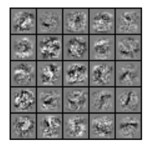
1.3 隐藏层可视化

结果：

---

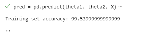
1.4 代码正确率

运行结果：

---

2 支持向量机（Support Vector Machines）

支持向量机：监督学习算法，广泛地应用于工业界和学术界。
从逻辑回归开始展示我们如何一点一点修改来得到本
质上的支持向量机。

---

2.1 优化目标

从逻辑回归开始

为了解释一些数学知识，我将用$z$ 表示${\theta }^{T}x$
z远远大于0的时候，即假设函数大于0.5且趋近于1，我们预测为1。
z远远小于0的时候，即假设函数小于0.5且趋近于0，我们预测为0。

代价函数的图像表示：

左下角的图：
当$y=1$时，此时在目标函数中只需有第一项起作用，我们得到 $y=-\log (\frac{1}{1+e^{-z}})$的图像如左下角所示，横坐标为$z={\theta }^{T}x$。当$z$越接近正无穷大，$h$越接近于1，代价越接近0。
将该图像换成紫色线就是SVM的表达式。表示，只要$z$的值大于1，代价就是0。
右下角的图：
当$y=0$时，此时在目标函数中只需有第二项起作用，我们得到 $y=-\log (1-\frac{1}{1+e^{-z}})$的图像如右下角所示，横坐标为$z={\theta }^{T}x$。当$z$越接近负无穷大，$h$越接近于0，代价越接近0。
同理，将该图像换成紫色线就是SVM的表达式。表示，只要$z$的值小于-1，代价就是0。
左边的函数，我称之为$\cos t_1(z)$，同时，右边函数我称它为$\cos t_0(z)$，下角标表示$y$的取值。

代价函数（与逻辑回归对比理解）

改动1：
$-\log (h_{\theta }(x^{(i)}))$改成：$\cos t_1({\theta }^{T}x)$，$-\log (1-h_{\theta }(x^{(i)}))$改成：$\cos t_0({\theta }^{T}x)$。
改动2：
式子乘以$m$，除以$\lambda$，用C代替$\frac{1}{\lambda }$
C越大，正则项就越可以忽略，容易过拟合。
C越小，正则项越重要，容易参数全为0，即差拟合。

总结：SVM的代价函数和假设函数

${\theta }^{T}x$大于0，我们就可以预测为1，但是为了使代价更小，我们希望${\theta }^{T}x$大于1。
${\theta }^{T}x$小于0，我们就可以预测为0，但是为了使代价更小，我们希望${\theta }^{T}x$小于-1。

---

2.2 大间距分类器（large margin ）

支持向量机将会选择这个黑色的决策边界，相较于之前我用粉色或者绿色画的决策界。这条黑色的看起来好得多，黑线看起来是更稳健的决策界。

当C太大的时候，SVM容易受异常点的影响而产生过拟合现象，因此，合理选择C的大小是很重要的。

---

2.4 核函数

之前讨论的SVM只能解决线性问题，为解决复杂的非线性问题，可以使用一种称为核的东西。
特征的选择

为了获得上图所示的非线性判定边界，我们的模型可能是$${\theta }_0+{\theta }_1{x}_1+{\theta }_2{x}_2+{\theta }_3{x}_1{x}_2+{\theta }_4{x}_1^2+{\theta }_5{x}_2^2+\cdots$$的形式。
我们可以用一系列的新的特征$f$来替换模型中的每一项。例如令：$$f_0=1,f_1=x_1,f_2=x_2,f_3=x_1{x}_2,f_4=x_1^2,f_5=x_2^2$$得到$$h_{\theta }(x)={\theta }_0{f}_0+{\theta }_1{f}_1+{\theta }_2{f}_2+...+{\theta }_n{f}_n$$然而，除了对原有的特征进行组合以外，有没有更好的方法来构造$f_1,f_2,f_3$？我们可以利用核函数来计算出新的特征。

高斯核函数

$x$:训练样本
$l^{(1)},l^{(2)},l^{(3)}$:地标
我们利用$x$的各个特征与我们预先选定的地标(landmarks)$l^{(1)},l^{(2)},l^{(3)}$的近似程度（similarity）来选取新的特征$f_1,f_2,f_3$。
$$f_1=similarity(x,l^{(1)})=\exp (-\frac{{\Vert x-l^{(1)}\Vert }^2}{2{\sigma }^2})$$,其中$${\Vert x-l^{(1)}\Vert }^2=\sum {}_{j=1}^n{(x_j-l_j^{(1)})}^2$$,为实例$x$中所有特征与地标$l^{(1)}$之间的距离的和。
上例中的$similarity(x,l^{(1)})$就是核函数，具体而言，这里是一个高斯核函数,记作：$k(x,l^{(i)})$。

地标的作用

如果一个训练样本$x$与地标$l$之间的距离近似于0，则新特征 $f$近似于$e^{-0}=1$，如果训练样本$x$与地标$l$之间距离较远，则$f$近似于$e^{-\infty }=0$

$\sigma$
假设我们的训练样本含有两个特征[$x_1$ $x{}_2$]，给定地标$l^{(1)}=\left[\begin{array}{c}3\\ 4\end{array}\right]$与不同的$\sigma$值:

图中水平面的坐标为 $x_1$，$x_2$，而垂直坐标轴代表$f$。可以看出，只有当$x$与$l^{(1)}$重合时$f$才具有最大值。随着$x$的改变$f$值改变的速率受到${\sigma }^2$的控制，${\sigma }^2$越大，速率越小。

假设${\theta }_0=-0.5,{\theta }_1=1,{\theta }_2=1,{\theta }_3=0$。
当样本处于洋红色的点位置处，因为其离$l^{(1)}$更近，但是离$l^{(2)}$和$l^{(3)}$较远，因此$f_1$接近1，而$f_2$,$f_3$接近0。因此$h_{\theta }(x)={\theta }_0+{\theta }_1{f}_1+{\theta }_2{f}_2+{\theta }_1{f}_3>0$，因此预测$y=1$。
同理可以求出，对于离$l^{(2)}$较近的绿色点，也预测$y=1$。
对于蓝绿色的点，因为其离三个地标都较远，预测$y=0$。
这样，图中红色的封闭曲线所表示的范围，便是我们的判定边界。

---

2.5 地标选取

地标选取及参数定义

(1)我们通常是根据训练集的数量选择地标的数量，即如果训练集中有$m$个样本，则我们选取$m$个地标，并且:$$l^{(1)}=x^{(1)},l^{(2)}=x^{(2)},.....,l^{(m)}=x^{(m)}$$这样做的好处在于：现在我们得到的新特征是建立在原有特征与训练集中所有其他特征之间距离的基础之上的。

(2)给定输入$x$，则定义：
$$\begin{gathered} f_0=1 \\ {f}_1=similarity(x,l^{(1)}) \\ {f}_2=similarity(x,l^{(2)}) \\ ... \end{gathered}$$定义向量$f$：$$f=\left[\begin{array}{c}{f}_0\\ f_1\\ f_2\\ ...\\ f_m\end{array}\right]$$其中$m$表示训练集的样本个数,$f_0=1$。

(3)给定训练样本$(x^{(i)},y^{(i)})$，其中$x^{(i)}$是n+1维的向量。则定义：
$$\begin{gathered} f_0^{(i)}=1 \\ {f}_1^{(i)}=similarity(x^{(i)},l^{(1)}) \\ {f}_2^{(i)}=similarity(x^{(i)},l^{(2)}) \\ {f}_i^{(i)}=similarity(x^{(i)},l^{(i)})=similarity(x^{(i)},x^{(i)})=1 \\ ... \end{gathered}$$定义向量$f^{(i)}$：$$f^{(i)}=\left[\begin{array}{c}{f}_0^{(i)}\\ f_1^{(i)}\\ f_2^{(i)}\\ ...\\ f_m^{(i)}\end{array}\right]$$其中$m$表示训练集的样本个数,$f_0^{(i)}=1$。
使用核函数的SVM

① 给定$x$，计算新特征$f$，当${\theta }^{T}f>=0$ 时，预测 $y=1$，否则反之。
② 相应地修改代价函数为：
$$minC\sum _{i=1}^m[y^{(i)}cos{t}_1({\theta }^T{f}^{(i)})+(1-y^{(i)})cos{t}_0({\theta }^T{f}^{(i)})]+\frac{1}{2}\sum _{j=1}^{n=m}{\theta }_j^2$$相比于之前的SVM的公式，将 ${\theta }^T{x}^{(i)}$改为了${\theta }^T{f}^{(i)}$。并且在SVM中，是有n个特征，在这里n也就是m，特征数等于样本数。
③ 对正则项进行调整：在计算$\sum _{j=1}^{n=m}{\theta }_j^2={\theta }^T\theta$时，我们用${\theta }^{T}M\theta$代替${\theta }^T\theta$，其中$M$是根据我们选择的核函数而不同的一个矩阵。这样做的原因是为了简化计算。

注意事项：
① 使用 $M$来简化计算的方法不适用于逻辑回归，因为计算将非常耗费时间。
② 我们不介绍最小化支持向量机的代价函数的方法，你可以使用现有的软件包（如liblinear,libsvm等）。在使用这些软件包最小化我们的代价函数之前，我们通常需要编写核函数。
③ 如果我们使用高斯核函数，那么在使用之前进行特征缩放是非常必要的。
④ 支持向量机也可以不使用核函数，不使用核函数又称为线性核函数(linear kernel)。
⑤ 当我们不采用非常复杂的函数，或者我们的训练集特征非常多（n很大）而样本非常少（m很小）的时候，可以采用这种不带核函数的支持向量机。
参数影响
$C=1/\lambda$
$C$ 较大时，相当于$\lambda$较小，正则项约等于没有，可能会导致过拟合，高方差；
$C$ 较小时，相当于$\lambda$较大，正则项过大，所有$\theta$会趋向于-，可能会导致差拟合，高偏差；

$\sigma$较大时，核函数就比较平滑，随着x的输入，变化也比较小，可能会导致低方差，高偏差（差拟合）；
$\sigma$较小时，核函数变化剧烈，可能会导致低偏差，高方差（过拟合）。

---

2.6 使用SVM

① 使用软件库，比如：liblinear和libsvm来求解参数$\theta$。
② 使用SVM需要解决两个问题：参数C的选择和核的选择。
不使用核函数（即线性核函数）：一般在n很大，m很小的时候使用。（因为样本m很小，只有少量的样本，那么决策边界可以用线来划分）
高斯核函数：需要确定参数${\sigma }^2$。

为什么选择高斯核函数

当n很小而m很大的时候：
假设n=2，m远远大于2，那么如上图所示。决策边界是一个很复杂的曲线，那么就需要用高斯核函数。

高斯核函数

① 使用SVM软件包之前，你可能需要先编写核函数代码。
② 在使用高斯核函数之前，需要先将特征归一化处理。

多分类问题

方法一：通常在软件包的内部已经内置好了多分类的代码，无需再写。
方法二：像之前的多分类算法一样，对于$y=1$训练出${\theta }^{(1)}$，$y=2$训练出${\theta }^{(2)}$…，最后选择最大的即可。

SVM和逻辑回归

$n$为特征数，$m$为训练样本数。
(1)如果相较于$m$而言，$n$要大许多，即训练集数据量不够支持我们训练一个复杂的非线性模型，我们选用逻辑回归模型或者不带核函数的支持向量机。
(2)如果$n$较小，而且$m$大小中等，例如$n$在 1-1000 之间，而$m$在10-10000之间，使用高斯核函数的支持向量机。
(3)如果$n$较小，而$m$较大，例如$n$在1-1000之间，而$m$大于50000，则使用支持向量机会非常慢，解决方案是创造、增加更多的特征，然后使用逻辑回归或不带核函数的支持向量机。

---

3 聚类

---

3.1 无监督学习

监督学习

无监督学习

---

3.2 k均值算法

k均值算法

K均值算法
K：簇的个数（即数据要分为几类）。
训练集：$x^{(1)},x^{(2)},...,x^{(m)}$，其中，$x^{(i)}$是n维的向量。
${\mu }^1$,${\mu }^2$,…,${\mu }^k$ 来表示聚类中心。
$c^{(1)}$,$c^{(2)}$,…,$c^{(m)}$来存储与第$i$个实例数据最近的聚类中心的索引。

随机初始化k个聚类中心：${\mu }^1$,${\mu }^2$,…,${\mu }^k$
第一个for循环是赋值步骤，即：对于每一个样例$i$，计算其应该属于的类。
第二个for循环是聚类中心的移动，即：对于每一个类$K$，重新计算该类的质心。

---

3.3 优化目标

K-均值最小化问题，是要最小化所有的数据点与其所关联的聚类中心点之间的距离之和，因此
K-均值的代价函数（又称畸变函数 Distortion function）为：
$$J(c^{(1)},...,c^{(m)},{\mu }_1,...,{\mu }_K)=\frac{1}{m}\sum _{i=1}^m{\Vert X^{\left(i\right)}-{\mu }_{c^{(i)}}\Vert }^2$$其中${\mu }_{c^{(i)}}$代表与$x^{(i)}$最近的聚类中心点。
我们的的优化目标便是找出使得代价函数最小的 $c^{(1)}$,$c^{(2)}$,…,$c^{(m)}$和${\mu }^1$,${\mu }^2$,…,${\mu }^k$。

${\mu }^1$,${\mu }^2$,…,${\mu }^k$ 来表示聚类中心。
$c^{(1)}$,$c^{(2)}$,…,$c^{(m)}$来存储与第$i$个实例数据最近的聚类中心的索引。

---

3.4 随机初始化

1. 我们应该选择$K<m$，即聚类中心点的个数要小于所有训练集实例的数量。
2. 随机选择$K$个训练实例，然后令$K$个聚类中心分别与这$K$个训练实例相等。

K-均值的一个问题在于，它有可能会停留在一个局部最小值处，而这取决于初始化的情况。
为了解决这个问题，我们通常需要多次运行**K-均值**算法，每一次都重新进行随机初始化，最后再比较多次运行**K-均值**的结果，选择代价函数最小的结果。这种方法在$K$较小的时候还是可行的，但是如果$K$较大，这么做也可能不会有明显地改善。

---