CS231n-assignment3-Network_Visualization(Pytorch)

在本笔记本中，我们将探索使用图像梯度生成新图像。

这里我们要做一些稍微不同的事情。我们将从一个卷积神经网络模型开始，该模型已经经过了对ImageNet数据集进行图像分类的预训练。我们将使用这个模型来定义一个损失函数，该函数量化我们当前对图像的不满意，然后使用反向传播来计算这个损失相对于图像像素的梯度。然后我们将保持模型不变，并对图像进行梯度下降，以合成新的图像，使损失最小化。

在本笔记本中，我们将探索三种图像生成技术:

显著性映射:显著性映射是一种快速的方法，可以告诉哪些部分的图像影响了网络的分类决策。

欺骗图像:我们可以干扰输入图像，使其在人类看来是一样的，但会被预先训练的网络错误分类。

类可视化:我们可以合成一幅图像，使特定类的分类分数最大化;这可以给我们一些感觉，当网络对这类图像进行分类时，它在寻找什么。

ln[1]:

import torch
import torchvision
import torchvision.transforms as T
import random
import numpy as np
from scipy.ndimage.filters import gaussian_filter1d
import matplotlib.pyplot as plt
from cs231n.image_utils import SQUEEZENET_MEAN, SQUEEZENET_STD
from PIL import Image

#%matplotlib inline
plt.rcParams['figure.figsize'] = (10.0, 8.0) # set default size of plots
plt.rcParams['image.interpolation'] = 'nearest'
plt.rcParams['image.cmap'] = 'gray'

Pretrained模型

对于我们所有的图像生成实验，我们将从一个卷积神经网络开始，该神经网络经过预先训练，可以在ImageNet上进行图像分类。在这里，我们可以使用任何模型，但为了实现这个任务，我们将使用SqueezeNet，它的精确度与AlexNet相当，但参数计数和计算复杂性显著降低。

SqeezeNet在ImageNet上实现了和AlexNet相同的正确率，但是只使用了1/50的参数。更进一步，使用模型压缩技术，可以将SqueezeNet压缩到0.5MB，这是AlexNet的1/510

一个Fire模块包括: 一个squeeze层 (只有1x1 卷积), 将其放入一个具有1x1 和3x3 卷积组合的expand层
使用SqueezeNet而不是AlexNet或VGG或ResNet意味着我们可以轻松地在CPU上执行所有图像生成实验。

ln[2]:

# Download and load the pretrained SqueezeNet model.
model = torchvision.models.squeezenet1_1(pretrained=True)

# We don't want to train the model, so tell PyTorch not to compute gradients
# with respect to model parameters.
for param in model.parameters():
    param.requires_grad = False
    
# you may see warning regarding initialization deprecated, that's fine, please continue to next steps

加载一些ImageNet图像

我们提供了一些来自ImageNet ILSVRC 2012分类数据集验证集的示例图像。要下载这些映像，请进入cs231n/datasets/并运行get_imagenet_val.sh。
由于它们来自验证集，我们的预训练模型在训练期间没有看到这些图像。
运行以下单元格以可视化其中一些图像，以及它们的ground-truth标签。

ln[3]:

from cs231n.data_utils import load_imagenet_val
X, y, class_names = load_imagenet_val(num=5)

plt.figure(figsize=(12, 6))
for i in range(5):
    plt.subplot(1, 5, i + 1)
    plt.imshow(X[i])
    plt.title(class_names[y[i]])
    plt.axis('off')
plt.gcf().tight_layout()

Saliency Maps
Saliency Maps告诉我们图像中的每个像素对该图像分类评分的影响程度。为了计算它，我们计算对应于正确类(这是一个标量)的非归一化分数的梯度相对于图像的像素。如果图像有形状(3,H, W)，那么这个梯度也会有形状(3,H, W);对于图像中的每个像素，这个梯度告诉我们，如果像素变化很小，分类评分将发生多大的变化。为了计算显著性图，我们取梯度的绝对值，然后取3个输入通道上的最大值;最终的Saliency Maps因此具有形状(H, W)，并且是非负的。

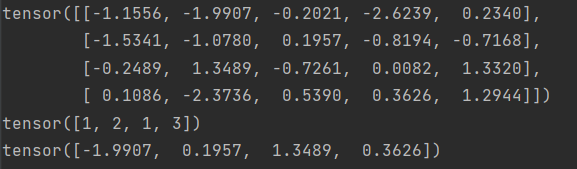
提示:PyTorch gather 方法
记得在作业1中你需要从矩阵的每一行中选择一个元素;如果s是一个numpy数组(N，C)和y是一个numpy数组(N，)其中0<=y[i]<C,那么s[np.arange(N), y)是一个numpy数组(N，),使用y中的下标从s中的每个元素中选择一个元素

在PyTorch中，您可以使用gather()方法执行相同的操作。如果s是形状(N, C)的PyTorch张量，y是形状(N，)的PyTorch张量，其长度范围为0 <= y[i] < C，则
s.gather (1，y.view(-1,1)) .squeeze () 是一个形状为(N，)的PyTorch张量，使用y中的下标从s中的每一行元素中选择一个元素

运行以下单元格以查看示例。

ln[4]:

# Example of using gather to select one entry from each row in PyTorch
def gather_example():
    N, C = 4, 5
    s = torch.randn(N, C)
    y = torch.LongTensor([1, 2, 1, 3])
    print(s)
    print(y)
    print(s.gather(1, y.view(-1, 1)).squeeze())
gather_example()

在cs231n/net_visualization_py实现compute_saliency_maps函数

def compute_saliency_maps(X, y, model):
    """
    Compute a class saliency map using the model for images X and labels y.

    Input:
    - X: Input images; Tensor of shape (N, 3, H, W)
    - y: Labels for X; LongTensor of shape (N,)
    - model: A pretrained CNN that will be used to compute the saliency map.

    Returns:
    - saliency: A Tensor of shape (N, H, W) giving the saliency maps for the input
    images.
    """
    # Make sure the model is in "test" mode
    model.eval()
    
    # Make input tensor require gradient
    X.requires_grad_()
    
    saliency = None
    ##############################################################################
    # TODO: Implement this function. Perform a forward and backward pass through #
    # the model to compute the gradient of the correct class score with respect  #
    # to each input image. You first want to compute the loss over the correct   #
    # scores (we'll combine losses across a batch by summing), and then compute  #
    # the gradients with a backward pass.                                        #
    ##############################################################################
    # *****START OF YOUR CODE (DO NOT DELETE/MODIFY THIS LINE)*****

    scores=model(X)
    scores=scores.gather(1,y.view(-1,1)).squeeze()
    scores.backward(torch.FloatTensor([1.0,1.0,1.0,1.0,1.0]))
    saliency=X.grad.data
    saliency=saliency.abs()
    saliency,i=torch.max(saliency,dim=1)
    saliency=saliency.squeeze()
    
    # *****END OF YOUR CODE (DO NOT DELETE/MODIFY THIS LINE)*****
    ##############################################################################
    #                             END OF YOUR CODE                               #
    ##############################################################################
    return saliency

ln[5]:

def show_saliency_maps(X, y):
    # Convert X and y from numpy arrays to Torch Tensors
    X_tensor = torch.cat([preprocess(Image.fromarray(x)) for x in X], dim=0)
    y_tensor = torch.LongTensor(y)

    # Compute saliency maps for images in X
    saliency = compute_saliency_maps(X_tensor, y_tensor, model)

    # Convert the saliency map from Torch Tensor to numpy array and show images
    # and saliency maps together.
    saliency = saliency.numpy()
    N = X.shape[0]
    for i in range(N):
        plt.subplot(2, N, i + 1)
        plt.imshow(X[i])
        plt.axis('off')
        plt.title(class_names[y[i]])
        plt.subplot(2, N, N + i + 1)
        plt.imshow(saliency[i], cmap=plt.cm.hot)
        plt.axis('off')
        plt.gcf().set_size_inches(12, 5)
    plt.show()

show_saliency_maps(X, y)

内联问题
你的一个朋友建议，为了找到最大化正确分数的图像，我们可以对输入图像执行梯度上升，但实际上我们可以在每个步骤中使用Saliency Maps来更新图像，而不是梯度。这个断言是正确的吗?
错误的，Saliency Maps只有正的值，所有都被计数为绝对值。

Fool image
我们还使用图像梯度来生成“欺骗图像”。给定一幅图像和一个目标类，我们可以对图像进行梯度爬升以最大化目标类，当网络将该图像分类为目标类时停止。实现以下函数来生成欺骗图像。
在cs231n/ net_visualization_py中实现make_fooling_image函数

def make_fooling_image(X, target_y, model):
    """
    Generate a fooling image that is close to X, but that the model classifies
    as target_y.

    Inputs:
    - X: Input image; Tensor of shape (1, 3, 224, 224)
    - target_y: An integer in the range [0, 1000)
    - model: A pretrained CNN

    Returns:
    - X_fooling: An image that is close to X, but that is classifed as target_y
    by the model.
    """
    # Initialize our fooling image to the input image, and make it require gradient
    X_fooling = X.clone()
    X_fooling = X_fooling.requires_grad_()

    learning_rate = 1
    ##############################################################################
    # TODO: Generate a fooling image X_fooling that the model will classify as   #
    # the class target_y. You should perform gradient ascent on the score of the #
    # target class, stopping when the model is fooled.                           #
    # When computing an update step, first normalize the gradient:               #
    #   dX = learning_rate * g / ||g||_2                                         #
    #                                                                            #
    # You should write a training loop.                                          #
    #                                                                            #
    # HINT: For most examples, you should be able to generate a fooling image    #
    # in fewer than 100 iterations of gradient ascent.                           #
    # You can print your progress over iterations to check your algorithm.       #
    ##############################################################################
    # *****START OF YOUR CODE (DO NOT DELETE/MODIFY THIS LINE)*****

    for i in range(100):
        scores = model(X_fooling)
        _, index = scores.max(dim=1)
        if index == target_y:
            break
        target_score = scores[0, target_y]
        target_score.backward()
        im_grad = X_fooling.grad
        X_fooling.data += learning_rate * (im_grad / im_grad.norm())
        X_fooling.grad.zero_()

    # *****END OF YOUR CODE (DO NOT DELETE/MODIFY THIS LINE)*****
    ##############################################################################
    #                             END OF YOUR CODE                               #
    ##############################################################################
    return X_fooling

运行以下单元格生成一个欺骗图像。理想情况下，您应该一眼能看出原始图像和欺骗图像之间没有什么主要区别，而且网络现在应该对欺骗图像做出错误的预测。然而，如果你观察10倍放大后的原始图像和欺骗图像之间的差异，你应该会看到一些随机噪声。可以随意更改idx变量来探索其他映像。

ln[6]:

idx = 0
target_y = 6

X_tensor = torch.cat([preprocess(Image.fromarray(x)) for x in X], dim=0)
X_fooling = make_fooling_image(X_tensor[idx:idx+1], target_y, model)

scores = model(X_fooling)
assert target_y == scores.data.max(1)[1][0].item(), 'The model is not fooled!'

在生成欺骗图像之后，运行以下单元来可视化原始图像、欺骗图像以及它们之间的差异。

ln[7]:

X_fooling_np = deprocess(X_fooling.clone())
X_fooling_np = np.asarray(X_fooling_np).astype(np.uint8)

plt.subplot(1, 4, 1)
plt.imshow(X[idx])
plt.title(class_names[y[idx]])
plt.axis('off')

plt.subplot(1, 4, 2)
plt.imshow(X_fooling_np)
plt.title(class_names[target_y])
plt.axis('off')

plt.subplot(1, 4, 3)
X_pre = preprocess(Image.fromarray(X[idx]))
diff = np.asarray(deprocess(X_fooling - X_pre, should_rescale=False))
plt.imshow(diff)
plt.title('Difference')
plt.axis('off')

plt.subplot(1, 4, 4)
diff = np.asarray(deprocess(10 * (X_fooling - X_pre), should_rescale=False))
plt.imshow(diff)
plt.title('Magnified difference (10x)')
plt.axis('off')

plt.gcf().set_size_inches(12, 5)
plt.show()

类可视化
通过从随机噪声图像开始，对目标类进行梯度爬升，我们可以生成网络将识别为目标类的图像。
具体来说，让$I$是一个图像，让$y$是一个目标类。设$s_y(I)$为卷积网络对类$y$赋给图像$I$的分数;注意，这些是原始的未标准化的分数，而不是类的概率。我们希望生成一个图像$I^{\ast }$，通过解决问题为类$y$获得高分

$I^{\ast }=arg{\max }_I(s_y(I)-R(I)))$

其中$R$是一个(可能是隐式的)正则化器(注意argmax中$R(I)$的符号:我们希望最小化这个正则化项)。我们可以使用梯度爬升来解决这个优化问题，计算相对于生成的图像的梯度。我们将使用(显式的)L2正则化形式

$R(I)==|i{|}_2^2$

在下面的单元格中，完成create_class_visualization函数的实现。

def class_visualization_update_step(img, model, target_y, l2_reg, learning_rate):
    ########################################################################
    # TODO: Use the model to compute the gradient of the score for the     #
    # class target_y with respect to the pixels of the image, and make a   #
    # gradient step on the image using the learning rate. Don't forget the #
    # L2 regularization term!                                              #
    # Be very careful about the signs of elements in your code.            #
    ########################################################################
    # *****START OF YOUR CODE (DO NOT DELETE/MODIFY THIS LINE)*****

    score = model(img)
    score[0, target_y].backward()
    im_grad = img.grad
    im_grad -= 2 * l2_reg * img
    img.data += learning_rate * im_grad / im_grad.norm()
    img.grad.zero_()

    # *****END OF YOUR CODE (DO NOT DELETE/MODIFY THIS LINE)*****
    ########################################################################
    #                             END OF YOUR CODE                         #
    ########################################################################

def create_class_visualization(target_y, model, dtype, **kwargs):
    """
    Generate an image to maximize the score of target_y under a pretrained model.

    Inputs:
    - target_y: Integer in the range [0, 1000) giving the index of the class
    - model: A pretrained CNN that will be used to generate the image
    - dtype: Torch datatype to use for computations

    Keyword arguments:
    - l2_reg: Strength of L2 regularization on the image
    - learning_rate: How big of a step to take
    - num_iterations: How many iterations to use
    - blur_every: How often to blur the image as an implicit regularizer
    - max_jitter: How much to gjitter the image as an implicit regularizer
    - show_every: How often to show the intermediate result
    """
    model.type(dtype)
    l2_reg = kwargs.pop('l2_reg', 1e-3)
    learning_rate = kwargs.pop('learning_rate', 25)
    num_iterations = kwargs.pop('num_iterations', 100)
    blur_every = kwargs.pop('blur_every', 10)
    max_jitter = kwargs.pop('max_jitter', 16)
    show_every = kwargs.pop('show_every', 25)

    # Randomly initialize the image as a PyTorch Tensor, and make it requires gradient.
    img = torch.randn(1, 3, 224, 224).mul_(1.0).type(dtype).requires_grad_()

    for t in range(num_iterations):
        # Randomly jitter the image a bit; this gives slightly nicer results
        ox, oy = random.randint(0, max_jitter), random.randint(0, max_jitter)
        img.data.copy_(jitter(img.data, ox, oy))
        class_visualization_update_step(img, model, target_y, l2_reg, learning_rate)
        # Undo the random jitter
        img.data.copy_(jitter(img.data, -ox, -oy))

        # As regularizer, clamp and periodically blur the image
        for c in range(3):
            lo = float(-SQUEEZENET_MEAN[c] / SQUEEZENET_STD[c])
            hi = float((1.0 - SQUEEZENET_MEAN[c]) / SQUEEZENET_STD[c])
            img.data[:, c].clamp_(min=lo, max=hi)
        if t % blur_every == 0:
            blur_image(img.data, sigma=0.5)

        # Periodically show the image
        if t == 0 or (t + 1) % show_every == 0 or t == num_iterations - 1:
            plt.imshow(deprocess(img.data.clone().cpu()))
            class_name = class_names[target_y]
            plt.title('%s\nIteration %d / %d' % (class_name, t + 1, num_iterations))
            plt.gcf().set_size_inches(4, 4)
            plt.axis('off')
            plt.show()

    return deprocess(img.data.cpu())

ln[8]:

dtype = torch.FloatTensor
model.type(dtype)
target_y = 76 # Tarantula
out = create_class_visualization(target_y, model, dtype)

完成上面单元格中的实现后，运行以下单元格来生成狼蛛的图像:

在其他类上尝试你的类可视化!您还可以随意使用各种超参数来尝试和改进生成的图像的质量，但这不是必需的。
ln[9]:

target_y = np.random.randint(1000) #这个自己随意修改
print(class_names[target_y])
X = create_class_visualization(target_y, model, dtype)