Trigger Word Detection

本文分析吴恩达触发点检测实验背景知识，介绍keras使用基本知识，从本实验出发了解相关深度学习内容。

实验背景

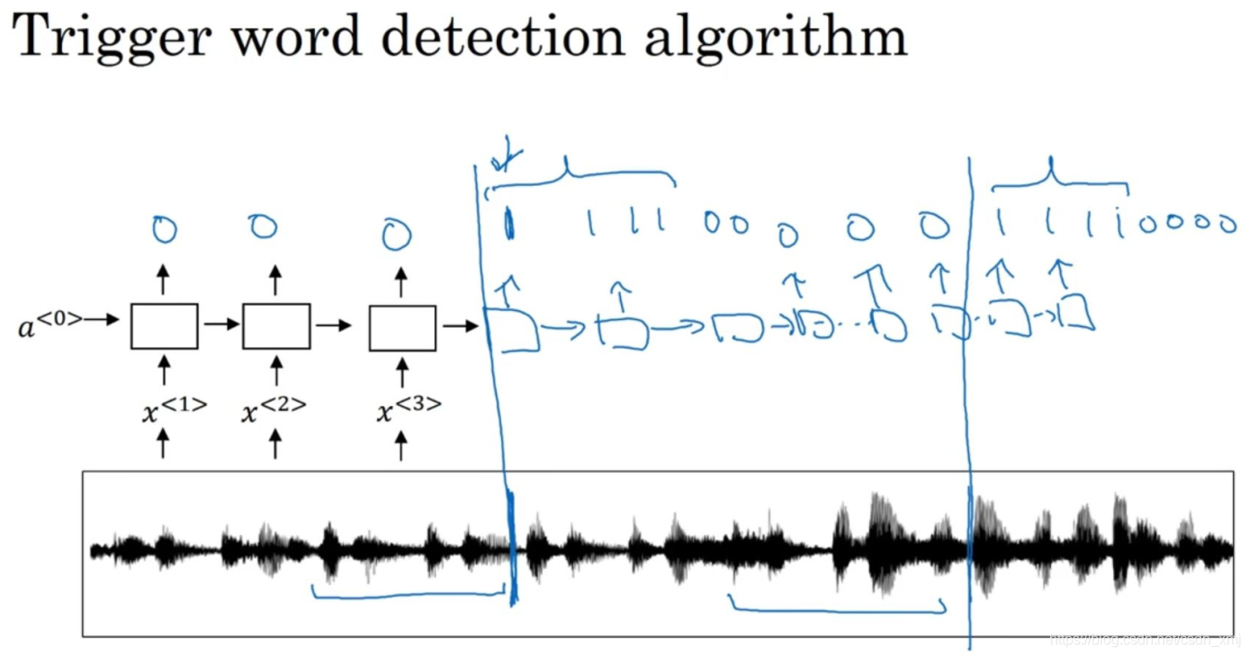
触发字检测

使用的是RNN结构，将音频片段（audio clip）处理成声谱图特征（spectrogram feathers），然后放入到rnn中，每当检测到目标后，标签设置为1，由于这种方法训练接不平衡，采用将目标出现一段时间后将一段标记为1；更容易训练；

实验过程

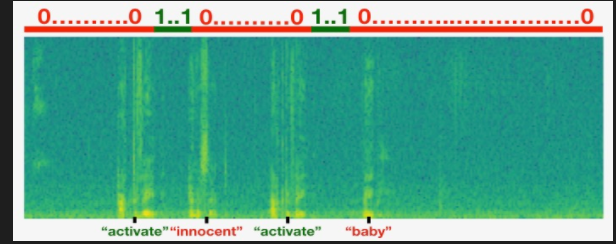
手工标记数据很难，人要去挺数据然后标记；采用合成方法，可以单独录制目标音频，噪音音频，负样本音频，然后将数据合成，自动生成标注，这样容易处理。

函数使用：

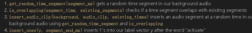
• 随机获取片段
• 是否已经合成（防止重叠）
• 合成
• label标记2

真实实验

采用真实数据训练保存；

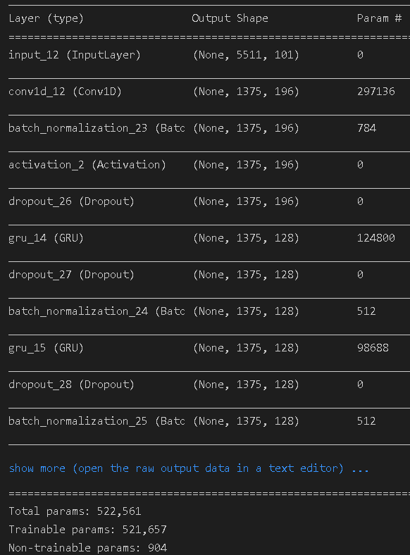
模型搭建：使用tensorflow1+keras:

# GRADED FUNCTION: model

def model(input_shape):
    """
    Function creating the model's graph in Keras.
    
    Argument:
    input_shape -- shape of the model's input data (using Keras conventions)

    Returns:
    model -- Keras model instance
    """
    
    X_input = Input(shape = input_shape)
    
    ### START CODE HERE ###
    
    # Step 1: CONV layer (≈4 lines)
    X = Conv1D(filters=196,kernel_size=15,strides=4)(X_input)                                # CONV1D
    X = BatchNormalization()(X)                                 # Batch normalization
    X = Activation(activation='relu')(X)                                 # ReLu activation
    X = Dropout(rate=0.8)(X)                                 # dropout (use 0.8)

    # Step 2: First GRU Layer (≈4 lines)
    X = GRU(units=128,return_sequences=True)(X)                                 # GRU (use 128 units and return the sequences)
    X = Dropout(rate=0.8)(X)                                 # dropout (use 0.8)
    X = BatchNormalization()(X)                                 # Batch normalization
    
    # Step 3: Second GRU Layer (≈4 lines)
    X = GRU(units=128,return_sequences=True)(X)                                 # GRU (use 128 units and return the sequences)
    X = Dropout(rate=0.8)(X)                                 # dropout (use 0.8)
    X = BatchNormalization()(X)                                 # Batch normalization
    X = Dropout(rate=0.8)(X)                                 # dropout (use 0.8)
    
    # Step 4: Time-distributed dense layer (≈1 line)
    X = TimeDistributed(Dense(1, activation = "sigmoid"))(X) # time distributed  (sigmoid)

    ### END CODE HERE ###

    model = Model(inputs = X_input, outputs = X)
    
    return model  

使用训练好的model（h5）：

model = load_model('./models/tr_model.h5')
opt = Adam(lr=0.0001, beta_1=0.9, beta_2=0.999, decay=0.01)
model.compile(loss='binary_crossentropy', optimizer=opt, metrics=["accuracy"])#加载模型 编译compile
model.fit(X, Y, batch_size = 5, epochs=1)
loss, acc = model.evaluate(X_dev, Y_dev)
print("Dev set accuracy = ", acc)

实验总结

用Keras构建神经网络的3种方法:

TensorFlow发展成为一个深度学习平台并不是一夜之间发生的。最初，TensorFlow将自己推销为一个符号数学库，用于跨一系列任务的数据流编程。因此，TensorFlow最初提供的主张并不是一个纯粹的机器学习库。目标是创建一个高效的数学库，以便在这种高效结构上构建的自定义机器学习算法能够在短时间内以高精度进行训练。

然而，用低级api重复地从头构建模型并不是很理想。因此，谷歌的工程师弗兰•库伊斯-克里特开发了Keras，作为一个独立的高层次的深度学习库。虽然Keras已经能够运行在不同的库之上，比如TensorFlow, Microsoft Cognitive Toolkit, Theano 或 PlaidML，但是TensorFlow过去和现在仍然是人们使用Keras的最常见的库。

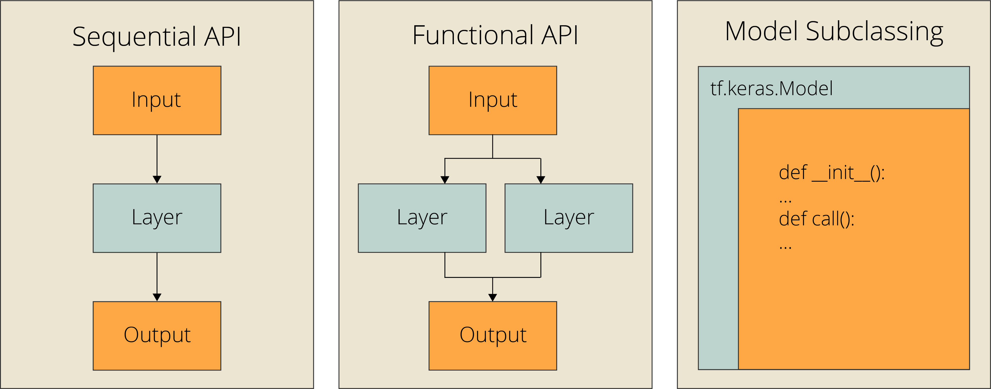
Sequential API

model = Sequential([ 
          Flatten(input_shape=(28, 28)), 
          Dense(256,'relu'), 
          Dense(10, "softmax"),
          ])

Functional API

inputs = Input(shape=(28, 28)) 
x = Flatten()(inputs) 
x = Dense(256, "relu")(x) 
outputs = Dense(10, "softmax")(x) 

model = Model(inputs=inputs, outputs=outputs, name="mnist_model")

模型子类化

class CustomModel(tf.keras.Model):

  def __init__(self, **kwargs):
    super(CustomModel, self).__init__(**kwargs)
    self.layer_1 = Flatten()
    self.layer_2 = Dense(256, "relu")
    self.layer_3 = Dense(10, "softmax")

  def call(self, inputs):
    x = self.layer_1(inputs)
    x = self.layer_2(x)
    x = self.layer_3(x)
    return x

model = CustomModel(name='mnist_model')

本次实验使用Functional 的方法。