python实现随机森林模型物种分布预测

前言

对于物种分布模型(SDM)，用的最多的无疑是最大熵模型（MaxEnt），它是基于最大化信息熵的原则，通过考虑已知的约束条件和最少的先验假设来推测物种在不同环境中的分布概率分布，本质上是一种先验概率假设方法。后来学者发现类似随机森林(RF)这种黑箱模型在物种分布预测过程中具有较好的效果。下面为python代码的实现过程。

基本思想

使用随机森林进行物种分布预测实际上以一个二分类问题，将物种分布点作为存在点（赋值1），将等数量的随机背景点作为不存在点（赋值0），再提取环境因子数据作为指标变量，建立随机森林分类模型，对整个区域所有位置进行物种存在概率计算。

数据准备

• 需要将物种分布坐标转换成shp数据，要求shp坐标与环境因子坐标一致
• 使用的所有指标变量要求投影以及分辨率一致
• 将研究区指标裁剪为一个矩形，这一步是因为我这样做的(成功了)，不知道不规则范围会不会出问题，小伙伴们可以自己试一试

需要的库

import geopandas as gpd
import numpy as np
import rasterio
import os
from sklearn.model_selection import train_test_split
from sklearn.ensemble import RandomForestClassifier
from sklearn.metrics import roc_auc_score, roc_curve, precision_score, recall_score, f1_score, accuracy_score
import matplotlib.pyplot as plt
from shapely.geometry import Point

加载物种点以及生成背景点

在生成背景点过程中为了防止生成的随机点与物种存在的位置重复，这里进行了筛选，使生成的背景点周围5km范围内没有物种点，由于物种分布点的数据为地理坐标系，所以我这里将其简单的转换成世界墨卡托投影来计算距离，这样就能避免生成的背景点读取的指标和物种分布点读取的指标一致，会对模型预测结果产生影响。

# 从shp文件中导入物种点数据
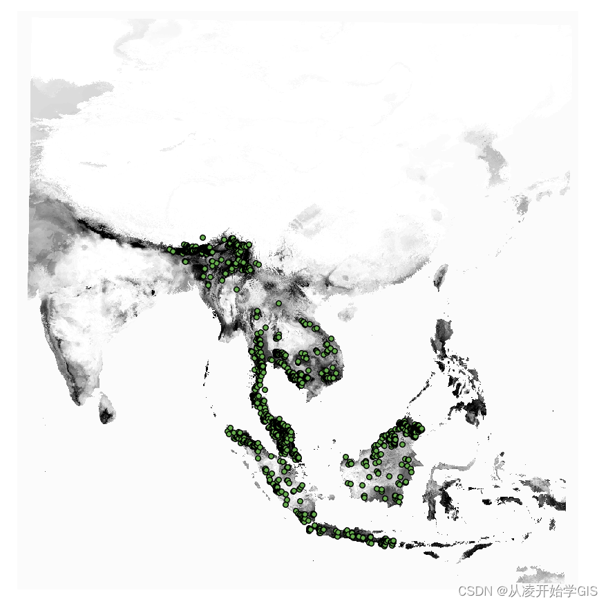
species_shp = gpd.read_file(r'F:\研究生\项目\犀鸟位点_8.6\犀鸟\process\souce\冠斑犀鸟.shp')
# 定义背景点函数(生成的背景点周围5km范围内没有物种点)
def generate_background_points(species, seed=None, buffer_distance=5000):
    bounding_box = species.total_bounds
    np.random.seed(seed)
    minx, miny, maxx, maxy = bounding_box
    # 将数据转换到世界墨卡托投影 (EPSG:3857)
    species_mercator = species.to_crs(epsg=3857)
    points = []
    for _ in range(len(species)):
        valid = False
        while not valid:
            x = np.random.uniform(minx, maxx)
            y = np.random.uniform(miny, maxy)
            point = Point(x, y)
            point_mercator = gpd.GeoSeries([point], crs=species.crs).to_crs(epsg=3857)[0]  # 转换点到墨卡托投影
            # 检查距离
            min_distance = species_mercator.distance(point_mercator).min()
            if min_distance >= buffer_distance:
                points.append(point)
                valid = True
    return gpd.GeoDataFrame({'geometry': points}, crs=species.crs)
# 生成背景点
background_points = generate_background_points(species_shp, seed=42, buffer_distance=5000)

定义值提取到点函数

def extract_values(points, raster_path):
    with rasterio.open(raster_path) as src:
        return [val[0] for val in src.sample(points['geometry'].apply(lambda geom: (geom.x, geom.y)))]

读取环境因子

# 从指定的目录自动获取所有的.tif文件
directory = r'F:\研究生\项目\犀鸟位点_8.6\犀鸟\process\处理过程数据\裁剪指标'
environmental_layers = [os.path.join(directory, file) for file in os.listdir(directory) if file.endswith('.tif')]
print("成功读取数据")
all_data = []
for layer in environmental_layers:
    species_values = extract_values(species_shp, layer)
    background_values = extract_values(background_points, layer)
    all_data.append(species_values + background_values)
print("读取物种点和背景点的环境指标并保存在data_matrix中")
data_matrix = np.array(all_data).T

去除异常值

这里我发现有的物种点的位置没有环境数据，我就将这部分的点删除了

print("去除异常值")
# 去除没有数值的点
nan_rows = np.any(np.isnan(data_matrix), axis=1)
data_matrix = data_matrix[~nan_rows]
labels = np.concatenate([np.ones(len(species_shp)), np.zeros(len(background_points))])[~nan_rows]

划分数据集并进行第一次训练

# 划分数据集
X_train, X_test, y_train, y_test = train_test_split(data_matrix, labels, test_size=0.3, random_state=42)
print("开始第一次训练")
# 训练随机森林模型
rf = RandomForestClassifier(n_estimators=100, random_state=42)
rf.fit(X_train, y_train)

计算特征重要性并可视化

# 计算特征重要性
feature_importances = rf.feature_importances_
feature_names = [os.path.basename(file).replace(".tif", "") for file in environmental_layers]
# 对特征重要性进行排序
sorted_idx = np.argsort(feature_importances)
# 绘制特征重要性条形图
plt.figure(figsize=(10, len(feature_names)))
plt.barh(range(len(feature_names)), feature_importances[sorted_idx])
plt.yticks(range(len(feature_names)), [feature_names[i] for i in sorted_idx])
plt.xlabel("Feature Importance")
plt.ylabel("Feature")
plt.title("Random Forest Feature Importance")
plt.tight_layout()
plt.show()

根据特征重要性筛选特征

一共19个环境因子，这里我选择了重要性排名前10的因子作为指标来建模

# 取重要性前10的特征
top_10_features = sorted_idx[-10:]
X_train = X_train[:, top_10_features]
X_test = X_test[:, top_10_features]
print("重新训练模型")
# 使用这些特征训练随机森林
rf.fit(X_train, y_train)
# 对测试集进行预测
y_pred_prob = rf.predict_proba(X_test)[:, 1]
y_pred = rf.predict(X_test)

模型评估

# 计算模型评估指标
accuracy = accuracy_score(y_test, y_pred)
auc = roc_auc_score(y_test, y_pred_prob)
precision = precision_score(y_test, y_pred)
recall = recall_score(y_test, y_pred)
f1 = f1_score(y_test, y_pred)

print(f"AUC: {auc:.4f}")
print(f"Precision: {precision:.4f}")
print(f"Recall: {recall:.4f}")
print(f"F1 Score: {f1:.4f}")
print(f"Accuracy: {accuracy:.4f}")

绘制ROC曲线

# 绘制ROC曲线
fpr, tpr, thresholds = roc_curve(y_test, y_pred_prob)
plt.figure()
plt.plot(fpr, tpr, label=f'ROC curve (AUC = {auc:.2f})')
plt.plot([0, 1], [0, 1], 'k--')
plt.xlabel('False Positive Rate')
plt.ylabel('True Positive Rate')
plt.title('ROC Curve')
plt.legend(loc="lower right")
plt.show()

至此，随机森林模型建立完成，其中我并没有对模型进行优化（因为我的模型效果很好），接下来只使用建立的模型对整个预测进行物种分布概率计算即可

预测数据准备

selected_layers = [environmental_layers[i] for i in top_10_features]

#  为整个范围生成坐标点
with rasterio.open(selected_layers[0]) as src:
    meta = src.meta
    width = src.width
    height = src.height
print("已读取预测范围")
x_coords = np.linspace(meta['transform'][2], meta['transform'][2] + meta['transform'][0] * width, width)
y_coords = np.linspace(meta['transform'][5], meta['transform'][5] + meta['transform'][4] * height, height)
coords = [(x, y) for y in y_coords for x in x_coords]
print("正在提取指标数值")
# 只对选中的特征文件提取相应的环境因子值
selected_data = []
for layer in selected_layers:
    print('正在读取{}指标数据'.format(layer))
    values = extract_values(gpd.GeoDataFrame({'geometry': [Point(x, y) for x, y in coords]}), layer)
    selected_data.append(values)
selected_data_matrix = np.array(selected_data).T

开始预测

print("开始预测")
# 使用已经训练好的模型对每个坐标点的物种存在概率进行预测
prediction_probs = rf.predict_proba(selected_data_matrix)[:, 1]
# 将预测的概率重新整理为与原始tif文件相同的维度
prediction_probs = prediction_probs.reshape((height, width))
# 使用 rasterio 保存预测的概率到新的 .tif 文件中
output_file = r"D:\FR\result\tif\predicted_distribution.tif"
with rasterio.open(output_file, 'w', **meta) as dst:
    dst.write(prediction_probs, 1)
print("预测结束!!!")

这个代码理解起来应该不难，但是由于我是代码菜鸡，运行起来很难！！！我的研究范围为大半个亚洲，空间分辨率为1km，模型已经建立成功，理论上只需要读取整个区域的指标数值，并保存为数组，然后就可以投喂给模型输出结果，然而，四个小时过后报错了。。。数据量太大了，数据存不下。但是如果研究区比较小或者电脑够强的话应该能运行成功，建议把数据存在固态硬盘里，根目录下，这种读取速度快一点。所以我就使用钞能力找人优化代码，果然，专业的事情还是要交给专业的人来完成，运行三分钟之后出结果了！！！我花了好久的时间，才东平西凑出来的抽象艺术，人家一下午就给我具体化了***，当然，大家有需要的话也可以给我回波血 * ~ *

优化后的代码流程如下：

• 加载数据
• 提取环境因子
• 数据预处理
• 划分数据集
• 使用所有特征训练RF模型
• 绘制特征重要性图
• 获取前10的重要特征
• 用PSO优化随机森林参数
• 使用优化的参数训练RF模型
  （不对模型进行优化）
• 评估模型
• 绘制ROC曲线
• 使用新模型进行区域预测
• 保存.tif文件
  完整代码运行时间在5~10min之间

代码主函数讲解

def main():
    print("加载数据~~~")
    species_shp = load_species_data()
    background_points = generate_background_points(species_shp, seed=42)
    environmental_layers = load_environmental_layers()

    print("提取环境因子")
    all_data = []
    for layer in environmental_layers:
        species_values = extract_values(species_shp, layer)
        background_values = extract_values(background_points, layer)
        all_data.append(species_values + background_values)
        #释放内存
        del species_values, background_values
        gc.collect()

    print("数据预处理")#数据整理
    data_matrix = np.array(all_data).T
    nan_rows = np.any(np.isnan(data_matrix), axis=1)
    data_matrix = data_matrix[~nan_rows]
    labels = np.concatenate([np.ones(len(species_shp)), np.zeros(len(background_points))])[~nan_rows]

    print("划分数据集")
    X_train, X_test, y_train, y_test = train_test_split(data_matrix, labels, test_size=0.3, random_state=42)

    print("使用所有特征训练RF模型")
    rf = train_rf(X_train, y_train, 100, None, 2, 1)

    print("绘制特征重要性图")
    plot_feature_importance(rf, environmental_layers)
    ## 这一步是用来筛选特征的，自己决定将重要性排名前几的指标作为预测特征
    print("获取前10的重要特征")
    top_indices, top_layers = get_top_features(rf, environmental_layers, 10)

    print("使用PSO优化随机森林参数")
    lb = [10, 1, 2, 1]#设置参数上限
    ub = [200, 30, 50, 20]#设置参数下限
    best_params, _ = pso(lambda params: objective_function(params, X_train, y_train, X_test, y_test, top_indices), lb,
                         ub, swarmsize=10, maxiter=10)

    optimal_n_estimators = int(best_params[0])
    optimal_max_depth = int(best_params[1]) if best_params[1] > 0 else None
    optimal_min_samples_split = int(best_params[2])
    optimal_min_samples_leaf = int(best_params[3])
    print("使用优化的参数训练RF模型")
    rf_top = train_rf(X_train[:, top_indices], y_train, optimal_n_estimators, optimal_max_depth,
                      optimal_min_samples_split, optimal_min_samples_leaf)
	
	## 若不需要优化模型则将上面优化部分的代码块注释，来运行下面的代码块
    # print("不对模型进行优化")
    # rf_top = train_rf(X_train[:, top_indices], y_train,100, None, 2, 1)

    print("评估模型")
    metrics, y_pred_prob = evaluate_model(rf_top, X_test[:, top_indices], y_test)
    for key, value in metrics.items():
        print(f"{key}: {value:.4f}")
    print("绘制ROC曲线")
    plot_roc_curve(y_test, y_pred_prob)
    
	## 这一步开始预测，训练好模型后将下面代码块解除注释后再运行。

   #  print("使用新模型进行区域预测")
   #  prediction_grid, meta = predict_on_grid(rf_top, top_layers)
   # 
   #  print("保存.tif文件")
   #  save_to_tif(prediction_grid, meta)
   # # 释放内存
   #  del prediction_grid,meta
   #  gc.collect()
   #  print("任务完成")

完整代码链接：https://x-x.fun/e/JZ0333abfdcxf	 

感谢大家花时间来阅读本文 作者水平有限 有失误之处请大家斧正！