以波士顿房价预测为例，演示过拟合问题和解决办法

极客李华

已于 2024-03-12 22:45:59 修改

阅读量1k

点赞数 28

分类专栏： AI 文章标签： ai

于 2024-03-04 22:12:35 首次发布

本文链接：https://blog.csdn.net/qq_51447496/article/details/136464193

版权

AI 专栏收录该内容

21 篇文章 3 订阅

订阅专栏

以波士顿房价预测为例，演示过拟合问题和解决办法

简介：以波士顿房价预测为例，演示过拟合问题和解决办法

作者简介：一名后端开发人员，每天分享后端开发以及人工智能相关技术，行业前沿信息，面试宝典。
座右铭：未来是不可确定的，慢慢来是最快的。
个人主页：极客李华-CSDN博客
合作方式：私聊+
这个专栏内容：用最低价格鼓励和博主一起在寒假打卡高频大厂算法题，连续一个月，提升自己的算法实力，为了算法比赛或者春招。
我的CSDN社区：https://bbs.csdn.net/forums/99eb3042821a4432868bb5bfc4d513a8
微信公众号，抖音，b站等平台统一叫做：极客李华，加入微信公众号领取各种编程资料，加入抖音，b站学习面试技巧，职业规划

首先需要在jupyter中安装对应的环境。

pip install numpy -i https://pypi.tuna.tsinghua.edu.cn/simple
pip install matplotlib -i https://pypi.tuna.tsinghua.edu.cn/simple
pip install pandas -i https://pypi.tuna.tsinghua.edu.cn/simple
pip install sklearn -i https://pypi.tuna.tsinghua.edu.cn/simple

1. 数据集介绍

使用Scikit-Learn库中的波士顿房价数据集，该数据集包含了房屋的各种特征以及相应的房价。

2. 模型选择

将使用简单的线性回归模型作为演示的基础模型，并尝试增加模型的复杂度以观察过拟合的情况。

3. 线性回归模型

线性回归模型的数学公式如下：

$y = w_0 + w_1x_1 + w_2x_2 + ... + w_nx_n$

其中， $y$ 是预测的房价， $x_i$ 是房屋的特征， $w_i$ 是特征的权重。

4. 实验步骤

a. 加载数据集并拆分训练集和测试集

from sklearn.datasets import load_boston
from sklearn.model_selection import train_test_split

# 加载波士顿房价数据集
boston = load_boston()
X = boston.data
y = boston.target

# 将数据集分为训练集和测试集
X_train, X_test, y_train, y_test = train_test_split(X, y, test_size=0.2, random_state=42)

b. 拟合线性回归模型

from sklearn.linear_model import LinearRegression
from sklearn.metrics import mean_squared_error

# 创建并拟合线性回归模型
model = LinearRegression()
model.fit(X_train, y_train)

# 在训练集和测试集上进行预测
train_predictions = model.predict(X_train)
test_predictions = model.predict(X_test)

# 计算均方误差（MSE）
train_mse = mean_squared_error(y_train, train_predictions)
test_mse = mean_squared_error(y_test, test_predictions)

print("训练集 MSE:", train_mse)
print("测试集 MSE:", test_mse)

c. 增加模型复杂度

为了演示过拟合的情况，我们可以增加模型的复杂度，比如使用多项式回归模型。

from sklearn.preprocessing import PolynomialFeatures
from sklearn.pipeline import make_pipeline

# 创建一个带有多项式特征的线性回归模型
degree = 10  # 可以尝试不同的多项式次数
model = make_pipeline(PolynomialFeatures(degree), LinearRegression())

# 拟合模型
model.fit(X_train, y_train)

# 在训练集和测试集上进行预测
train_predictions = model.predict(X_train)
test_predictions = model.predict(X_test)

# 计算均方误差（MSE）
train_mse = mean_squared_error(y_train, train_predictions)
test_mse = mean_squared_error(y_test, test_predictions)

print("训练集 MSE:", train_mse)
print("测试集 MSE:", test_mse)

完整代码

from sklearn.datasets import load_boston
from sklearn.model_selection import train_test_split
from sklearn.linear_model import LinearRegression
from sklearn.metrics import mean_squared_error
from sklearn.preprocessing import PolynomialFeatures
from sklearn.pipeline import make_pipeline

# 加载波士顿房价数据集
boston = load_boston()
X = boston.data
y = boston.target

# 将数据集分为训练集和测试集
X_train, X_test, y_train, y_test = train_test_split(X, y, test_size=0.2, random_state=42)

# 创建并拟合线性回归模型
model = LinearRegression()
model.fit(X_train, y_train)

# 在训练集和测试集上进行预测
train_predictions = model.predict(X_train)
test_predictions = model.predict(X_test)

# 计算均方误差（MSE）
train_mse = mean_squared_error(y_train, train_predictions)
test_mse = mean_squared_error(y_test, test_predictions)

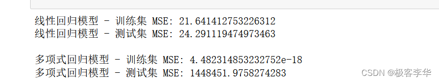
print("线性回归模型 - 训练集 MSE:", train_mse)
print("线性回归模型 - 测试集 MSE:", test_mse)

# 创建一个带有多项式特征的线性回归模型
degree = 10  # 可以尝试不同的多项式次数
model_poly = make_pipeline(PolynomialFeatures(degree), LinearRegression())

# 拟合多项式回归模型
model_poly.fit(X_train, y_train)

# 在训练集和测试集上进行预测
train_predictions_poly = model_poly.predict(X_train)
test_predictions_poly = model_poly.predict(X_test)

# 计算多项式回归模型的均方误差（MSE）
train_mse_poly = mean_squared_error(y_train, train_predictions_poly)
test_mse_poly = mean_squared_error(y_test, test_predictions_poly)

print("\n多项式回归模型 - 训练集 MSE:", train_mse_poly)
print("多项式回归模型 - 测试集 MSE:", test_mse_poly)


import matplotlib.pyplot as plt

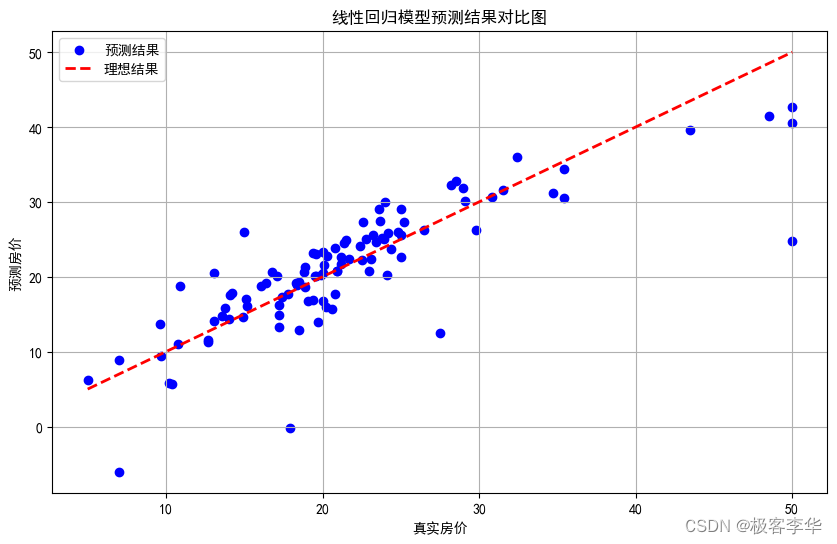
# 绘制线性回归模型的预测结果与真实结果对比图
plt.figure(figsize=(10, 6))
plt.scatter(y_test, test_predictions, color='blue', label='预测结果')
plt.plot([y_test.min(), y_test.max()], [y_test.min(), y_test.max()], 'k--', lw=2, color='red', label='理想结果')
plt.xlabel('真实房价')
plt.ylabel('预测房价')
plt.title('线性回归模型预测结果对比图')
plt.legend()
plt.grid(True)
plt.show()

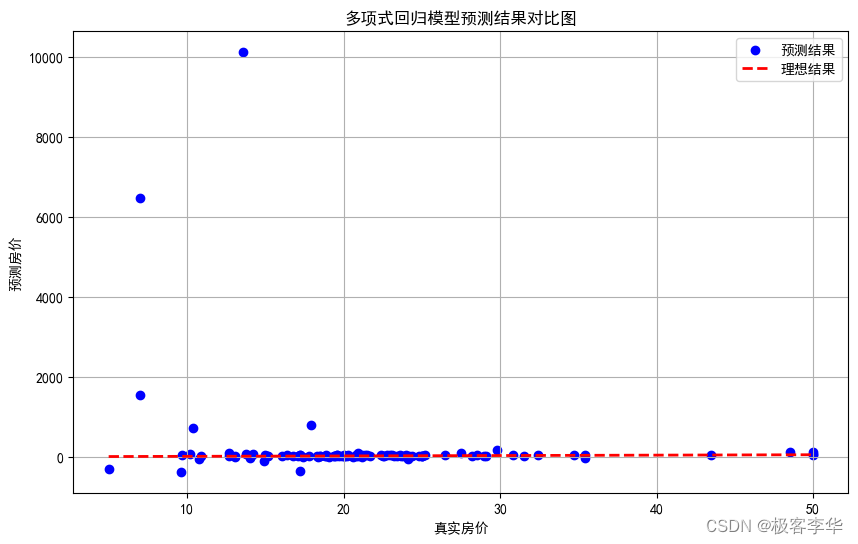
# 绘制多项式回归模型的预测结果与真实结果对比图
plt.figure(figsize=(10, 6))
plt.scatter(y_test, test_predictions_poly, color='blue', label='预测结果')
plt.plot([y_test.min(), y_test.max()], [y_test.min(), y_test.max()], 'k--', lw=2, color='red', label='理想结果')
plt.xlabel('真实房价')
plt.ylabel('预测房价')
plt.title('多项式回归模型预测结果对比图')
plt.legend()
plt.grid(True)
plt.show()

运行结果

在这里插入图片描述

运行结果分析

训练集MSE和测试集MSE之间的差异：
- 在线性回归模型中，训练集MSE和测试集MSE的差异不大，而在多项式回归模型中，训练集MSE非常小，但测试集MSE却非常大。
- 多项式回归模型在训练集上的MSE接近零，这表明模型可以完美地拟合训练数据，但在测试集上的MSE非常大，这表明模型在未见过的数据上表现很差，这是典型的过拟合现象。
多项式回归模型的测试集MSE异常地大：
- 测试集MSE达到了数百万的级别，这说明模型在测试集上的预测结果与真实值之间存在很大的偏差，模型的泛化能力非常差。
训练集MSE接近零：
- 多项式回归模型在训练集上的MSE非常接近零，这表明模型可以完美地拟合训练数据，甚至可能过度拟合了训练数据中的噪声和细节。

多项式回归模型在训练集上表现得很好，但在测试集上的表现非常糟糕，这是典型的过拟合现象。这种情况下，模型在训练集上过度拟合了数据，失去了泛化能力，不能很好地适应新的数据。为了解决过拟合问题，可以尝试降低模型的复杂度、增加数据量、进行特征选择或使用正则化等方法。

解决问题代码

常见的方法之一是使用正则化技术，特别是岭回归（Ridge Regression）或Lasso回归（Lasso Regression）。这些方法可以限制模型的复杂度，从而减少过拟合的风险。

岭回归模型和普通的线性回归模型之间的主要区别在于岭回归模型引入了L2正则化项，而普通的线性回归模型没有正则化项。

具体来说，岭回归模型在损失函数中添加了一个L2范数惩罚项，用于惩罚模型系数的大小。这个惩罚项可以防止模型过度拟合训练数据，因为它会使得模型系数更加稳定，减少模型对数据中噪声的敏感性。

岭回归模型的损失函数定义如下：

$\text{Loss} = \text{MSE} + \alpha \sum_{i=1}^{n} \beta_i^2$
其中，MSE表示均方误差， $\alpha$ 是正则化参数，用于控制正则化的强度， $\beta_i$ 表示模型的系数。

相比之下，普通的线性回归模型只优化MSE，没有引入正则化项。因此，在训练数据足够多的情况下，普通的线性回归模型可能会出现过拟合的问题。

岭回归模型相对于普通线性回归模型来说，更加稳健，能够更好地处理高维数据和多重共线性，减少模型的过拟合风险。

下面是改进后的代码，采用了岭回归来解决过拟合问题：

from sklearn.datasets import load_boston
from sklearn.model_selection import train_test_split
from sklearn.linear_model import Ridge
from sklearn.metrics import mean_squared_error
from sklearn.preprocessing import PolynomialFeatures
from sklearn.pipeline import make_pipeline

import matplotlib.pyplot as plt

# 加载波士顿房价数据集
boston = load_boston()
X = boston.data
y = boston.target

# 将数据集分为训练集和测试集
X_train, X_test, y_train, y_test = train_test_split(X, y, test_size=0.2, random_state=42)

# 创建并拟合岭回归模型
alpha = 1.0  # 正则化参数，可以调整
model_ridge = Ridge(alpha=alpha)
model_ridge.fit(X_train, y_train)

# 在训练集和测试集上进行预测
train_predictions_ridge = model_ridge.predict(X_train)
test_predictions_ridge = model_ridge.predict(X_test)

# 计算岭回归模型的均方误差（MSE）
train_mse_ridge = mean_squared_error(y_train, train_predictions_ridge)
test_mse_ridge = mean_squared_error(y_test, test_predictions_ridge)

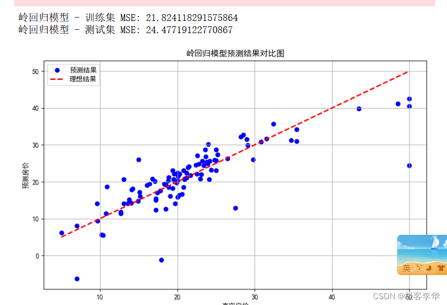
print("岭回归模型 - 训练集 MSE:", train_mse_ridge)
print("岭回归模型 - 测试集 MSE:", test_mse_ridge)

# 绘制岭回归模型的预测结果与真实结果对比图
plt.figure(figsize=(10, 6))
plt.scatter(y_test, test_predictions_ridge, color='blue', label='预测结果')
plt.plot([y_test.min(), y_test.max()], [y_test.min(), y_test.max()], 'k--', lw=2, color='red', label='理想结果')
plt.xlabel('真实房价')
plt.ylabel('预测房价')
plt.title('岭回归模型预测结果对比图')
plt.legend()
plt.grid(True)
plt.show()