[DeepLearning] 线性回归的实现Pytorch

[DeepLearning] 线性回归的实现Pytorch

欢迎大家访问我的GitHub博客

https://lunan0320.cn

线性回归从零开始实现

模块导入

%matplotlib inline 
import random
import torch
from d2l import torch as d2l

获取数据

def synthetic_data(w,b,num_examples):
    X = torch.normal(0,1,(num_examples,len(w)))
    y = torch.matmul(X,w) + b
    y += torch.normal(0,0.01,y.shape)
    return X, y.reshape((-1,1))

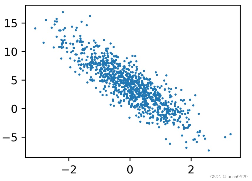
true_w = torch.tensor([2,-3.4])
true_b = 4.2
features, labels = synthetic_data(true_w,true_b,1000)

print('featrues:',features[0],'\n;abel:',labels[0])
features.shape,labels.shape

featrues: tensor([0.1349, 1.4104]) 
;abel: tensor([-0.311

(torch.Size([1000, 2]), torch.Size([1000, 1]))

d2l.set_figsize()
d2l.plt.scatter(features[:, (1)].detach().numpy(), labels.detach().numpy(), 1);

​

按batch分组

def data_iter(batch_size, features, labels):
    num_examples = len(features)
    indices = list(range(num_examples))
    #随机化打乱
    random.shuffle(indices)
    for i in range(0, num_examples,batch_size):
        batch_indices = torch.tensor(indices[i:min(i + batch_size, num_examples)])
        yield features[batch_indices],labels[batch_indices]

batch_size  = 10
for X, y in data_iter(batch_size,features,labels):
    print("x:",X,'\n y:',y)
    break

x: tensor([[ 0.4850,  0.4973],
        [-1.0981,  1.2369],
        [-0.1405, -1.2454],
        [ 0.8456,  0.3941],
        [ 0.0963,  0.2370],
        [ 0.2307, -1.1592],
        [ 0.7825,  0.0879],
        [ 0.7552,  0.9239],
        [ 1.6729,  1.4891],
        [ 0.5359, -0.2831]]) 
 y: tensor([[ 3.4988],
        [-2.2224],
        [ 8.1597],
        [ 4.5686],
        [ 3.5808],
        [ 8.6105],
        [ 5.4748],
        [ 2.5732],
        [ 2.4736],
        [ 6.2488]])

w = torch.normal(0,0.01,size=(2,1),requires_grad = True)
b = torch.zeros(1,requires_grad = True)

线性回归

def linreg(X,w,b):
    return torch.matmul(X,w) + b

平方误差损失函数

def squared_loss(y_hat,y):
    return (y_hat - y.reshape(y_hat.shape))**2 / 2

随机梯度下降

def sgd(params,lr, batch_size):
    with torch.no_grad():
        for param in params:
            param  -= lr * param.grad / batch_size
            param.grad.zero_()

迭代训练

lr = 0.03 
num_epochs = 3
net = linreg
loss = squared_loss
for epoch in range(num_epochs):
    for X, y in data_iter(batch_size, features, labels):
        l = loss(net(X, w, b), y)
        l.sum().backward()
        sgd([w,b], lr, batch_size)
    with torch.no_grad():
        train_l = loss(net(features, w, b),labels)
        print(f'epoch {epoch + 1}, loss{float(train_l.mean()):f}')

epoch 1, loss0.000050
epoch 2, loss0.000050
epoch 3, loss0.000050

print(f'w的估计误差:{true_w - w.reshape(true_w.shape)}')
print(f'b的估计误差;{true_b - b})')

w的估计误差:tensor([0.0002, 0.0005], grad_fn=<SubBackward0>)
b的估计误差;tensor([-0.0004], grad_fn=<RsubBackward1>))

线性回归的简洁实现（Pytorch框架）

import numpy as np
import torch
from torch.utils import data

#生成数据集
true_w = torch.tensor([2,-3.4])
true_b = 4.2
def synthetic_data(w,b ,num_examples):
    X = torch.normal(0, 1, size=(num_examples,len(w)))
    y = torch.matmul(X, w) + b
    y += torch.normal(0,0.01,y.shape)
    return X, y.reshape(-1,1)
features,labels = synthetic_data(true_w,true_b,1000)
features.shape,labels.shape

(torch.Size([1000, 2]), torch.Size([1000, 1]))

#读取数据集
def load_array(datas,batch_size, is_train = True):
    dataset = data.TensorDataset(*datas)
    return data.DataLoader(dataset,batch_size,shuffle = is_train)
batch_size = 10
data_iter = load_array((features,labels),batch_size)

#定义模型
from torch import nn
#全连接层是Linear类，
net = nn.Sequential(nn.Linear(2,1))

初始化模型参数

在线性回归中需要初始化权重weight和偏置bias
此处：权重参数从均值为0，标准差为0.01的正态分布中随机采样，偏置参数初始化为0

#初始化参数
net[0].weight.data.normal_(0,0.01)
net[0].bias.data.fill_(0)

tensor([0.])

定义损失函数

平方误差在nn中是使用的MSELoss类，即平方L_{2}范数
默认情况下，返回的是所有样本loss的平均值

loss = nn.MSELoss()

定义优化算法

小批量梯度下降算法在PyTorch的optim模块下实现
可以指定要优化的超参数，此处只需要自己设置learning rate

trainer = torch.optim.SGD(net.parameters(),lr = 0.03)

训练

每个epoch，要完整遍历一次数据集train_data
对于每个mini_batch，执行：

• 过调用net(X)生成预测并计算损失l（前向传播）
• 通过进行反向传播来计算梯度。
• 调用优化器来更新模型参数

num_epochs = 3
for epoch in range(num_epochs):
    for X,y in data_iter:
        l = loss(net(X),y)
        trainer.zero_grad()
        l.backward()
        trainer.step()
    l = loss(net(features),labels)
    print(f'epoch{epoch+1},loss{l:f}')
    

epoch1,loss0.000102
epoch2,loss0.000102
epoch3,loss0.000101

w = net[0].weight.data
print('w的估计误差：', true_w - w.reshape(true_w.shape))
b = net[0].bias.data
print('b的估计误差：', true_b - b)

w的估计误差： tensor([0.0003, 0.0004])
b的估计误差： tensor([3.3379e-06])