机器学习（复试）

所有复试设计网站整理在复试文件夹中

学习分类

其学习形式主要分为：有监督学习、无监督学习、半监督学习

有监督

有监督学习（supervised learning），需要你事先需要准备好要输入数据（训练样本）与真实的输出结果（参考答案)

预测结果分类

比如有监督学习可以划分为：回归问题和分类问题
如果预测结果是离散的，通常为分类问题，而为连续的，则是回归问题。

机器学习的专业术语

1. 模型：模型这一词语将会贯穿整个教程的始末，它是机器学习中的核心概念。
2. 数据集
3. 样本&特征
4. 向量
5. 矩阵：矩阵看成由向量组成的二维数组

假设函数和损失函数

1. 假设函数：假设函数（Hypothesis Function）可表述为 y=f(x) 其中 x 表示输入数据，而 y 表示输出的预测结果
2. 损失函数：损失函数（Loss Function）又叫目标函数，简写为 L(x)，这里的 x 是假设函数得出的预测结果“y”，如果 L(x) 的返回值越大就表示预测结果与实际偏差越大，越小则证明预测值越来越“逼近”真实值，
3. 优化方法：“优化方法”可以理解为假设函数和损失函数之间的沟通桥梁。

拟合&过拟合&欠拟合

1)拟合：形象地说，“拟合”就是把平面坐标系中一系列散落的点，用一条光滑的曲线连接起来，因此拟合也被称为“曲线拟合”。
2) 过拟合：过拟合（overfitting）与是机器学习模型训练过程中经常遇到的问题，所谓过拟合，通俗来讲就是模型的泛化能力较差，也就是过拟合的模型在训练样本中表现优越，但是在验证数据以及测试数据集中表现不佳。过拟合问题在机器学习中经常遇到，主要是因为训练时样本过少，特征值过多导致的，后续还会详细介绍。
3) 欠拟合：欠拟合（underfitting）恰好与过拟合相反，它指的是“曲线”不能很好的“拟合”数据。

基本的人工智能工具的介绍与使用

详细介绍见复试文件夹中语雀文档

1 python

2 numpy (矩阵计算)

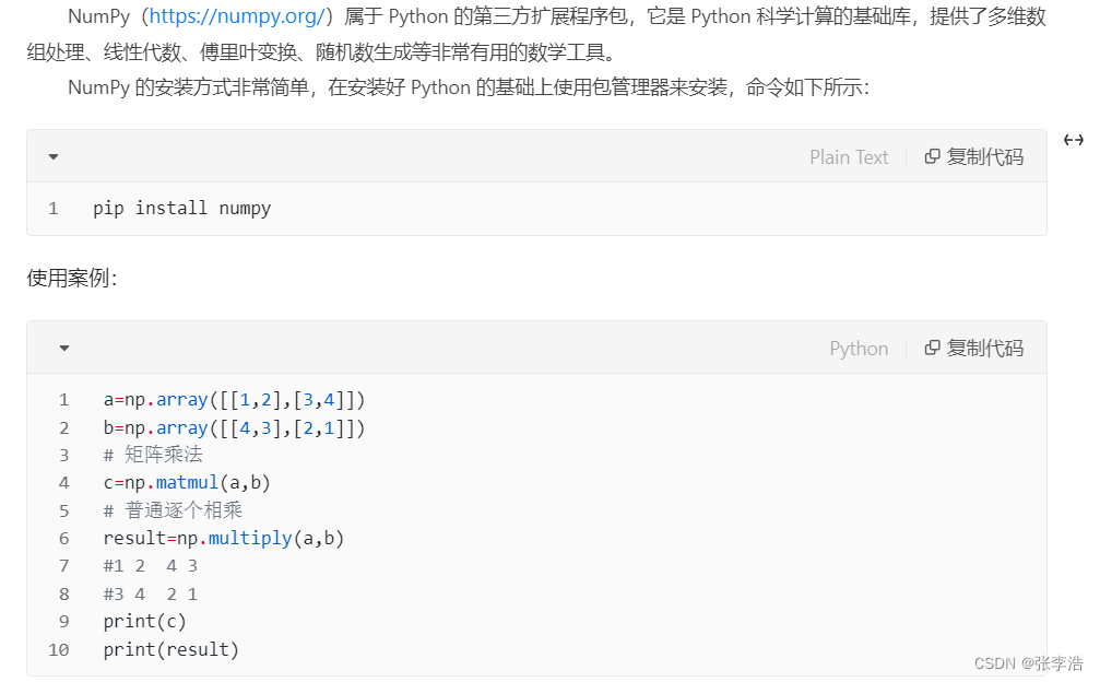
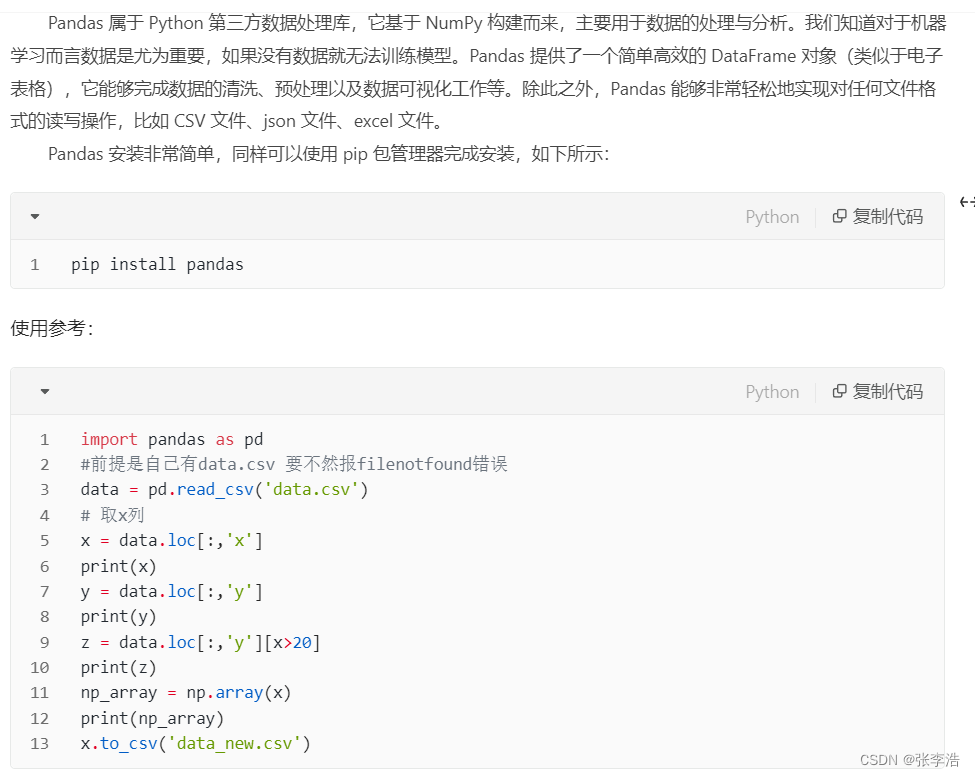
3 pandas（读取文件）

4 Matplotlib（数据可视化）

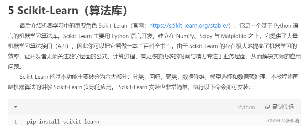
5 Scikit-Learn（算法库）

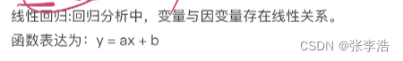
线性回归

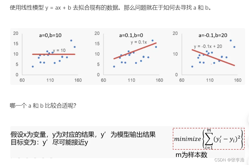
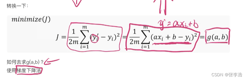
利用梯度下降法求极小值

计算的过程比较复杂且涉及数学公式
所以我简单总结一下：就是

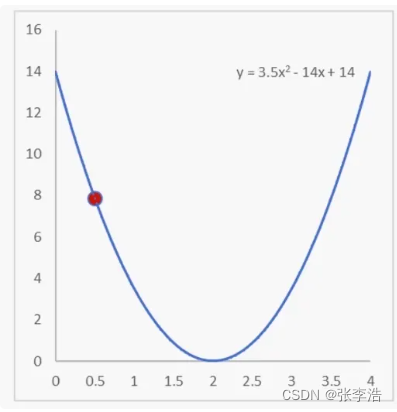
重复计算红点处的斜率，并通过不断的迭代，最终找到极小值

Sklearn求解线性回归问题

基于generated_data.csv数据，建立线性回归模型，预测x=3.5对应的y值，评估模型表现。
学会用Sklearn求解线性回归问题，寻找a、b (y = ax + b) 并且评估模型的好坏。
数据如下：

#加载数据
import pandas as pd
data = pd.read_csv('generated_data.csv')
data.head()
x = data.loc[:,'x']// 分别看下x和y的数值
y = data.loc[:,'y']
print(x,y)

#visualize the data
from matplotlib import pyplot as plt
plt.figure(figsize=(20,20))
plt.scatter(x,y)//绘制散点图
plt.show()

#set up a linear regression model // 建立线性回归模型
from sklearn.linear_model import LinearRegression
lr_model = LinearRegression()


import numpy as np
x = np.array(x)//转换为np的数组
x = x.reshape(-1,1)
y = np.array(y)
y = y.reshape(-1,1)

print(type(x),x.shape,type(y),y.shape)
print(type(x),x.shape)


lr_model.fit(x,y)//喂数据
y_predict = lr_model.predict(x)
print(y_predict)

y_3 = lr_model.predict([[3.5]])//预测x=3.5时y的数值
print(y_3)
print(y)

#a\b 打印
a = lr_model.coef_//a是斜率
b = lr_model.intercept_//b是截距
print(a,b)

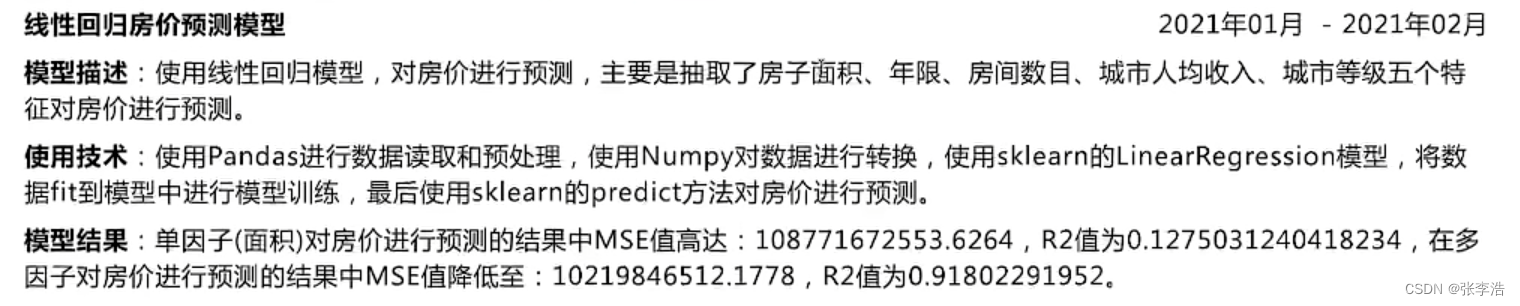
评估模型表现使用的指标

一、MSE
二、R^2

房价预测

# 加载数据
import pandas as pd
import numpy as np
data = pd.read_csv('usa_housing_price.csv')
data.head()


#数据散点图展示
%matplotlib inline
from matplotlib import pyplot as plt
fig = plt.figure(figsize=(10,10))
fig1 =plt.subplot(231)
plt.scatter(data.loc[:,'Avg. Area Income'],data.loc[:,'Price'])
plt.title('Price VS Income')

fig2 =plt.subplot(232)
plt.scatter(data.loc[:,'Avg. Area House Age'],data.loc[:,'Price'])
plt.title('Price VS House Age')

fig3 =plt.subplot(233)
plt.scatter(data.loc[:,'Avg. Area Number of Rooms'],data.loc[:,'Price'])
plt.title('Price VS Number of Rooms')

fig4 =plt.subplot(234)
plt.scatter(data.loc[:,'Area Population'],data.loc[:,'Price'])
plt.title('Price VS Area Population')

fig5 =plt.subplot(235)
plt.scatter(data.loc[:,'size'],data.loc[:,'Price'])
plt.title('Price VS size')
plt.show()

#定义 x 和 y
X = data.loc[:,'size']
y = data.loc[:,'Price']
y.head()

# 转换维度
X = np.array(X).reshape(-1,1)
print(X.shape)


#线性回归模型
from sklearn.linear_model import LinearRegression
LR1 = LinearRegression()
#训练模型
LR1.fit(X,y)

#预测
y_predict_1 = LR1.predict(X)
print(y_predict_1)

#模型评估
from sklearn.metrics import mean_squared_error,r2_score
mean_squared_error_1 = mean_squared_error(y,y_predict_1)
r2_score_1 = r2_score(y,y_predict_1)
print(mean_squared_error_1,r2_score_1)

# 绘图
fig6 = plt.figure(figsize=(8,5))
plt.scatter(X,y)
plt.plot(X,y_predict_1,'r')
plt.show()

#定义多因子x
#删除掉Price列
X_multi = data.drop(['Price'],axis=1)
X_multi

#第二个线性模型
LR_multi = LinearRegression()
#train the model
LR_multi.fit(X_multi,y)

#多因子预测
y_predict_multi = LR_multi.predict(X_multi)
print(y_predict_multi)

mean_squared_error_multi = mean_squared_error(y,y_predict_multi)
r2_score_multi = r2_score(y,y_predict_multi)
print(mean_squared_error_multi,r2_score_multi)

print(mean_squared_error_1)

fig7 = plt.figure(figsize=(8,5))
plt.scatter(y,y_predict_multi)
plt.show()

fig8 = plt.figure(figsize=(8,5))
plt.scatter(y,y_predict_1)
plt.show()

//输入5个数据的具体数值
X_test = [65000,5,5,30000,200]
X_test = np.array(X_test).reshape(1,-1)
print(X_test)

y_test_predict = LR_multi.predict(X_test)
print(y_test_predict)

简历制作

面试不会的问题

虽然这个不会但是我会。。。

项目介绍

自我介绍

仅供参考，比较随意，需要补充