解决分类问题的源代码

# 决策树
​​​​​

from sklearn import tree
X = [[0, 0], [1, 1]]
Y = [0, 1]

dt_test_clf = tree.DecisionTreeClassifier()
dt_test_clf = dt_test_clf.fit(X, Y)

dt_test_clf.predict([[2., 2.]])

array([1])
dt_test_clf.predict_proba([[2., 2.]])

array([[0., 1.]])
# 训练模型
from sklearn.datasets import load_iris
from sklearn import tree

iris = load_iris()
dt_clf = tree.DecisionTreeClassifier()
dt_clf = dt_clf.fit(iris.data, iris.target)

# 模型预测
y_pred = dt_clf.predict(iris.data)
y_pred

array([0, 0, 0, 0, 0, 0, 0, 0, 0, 0, 0, 0, 0, 0, 0, 0, 0, 0, 0, 0, 0, 0,
       0, 0, 0, 0, 0, 0, 0, 0, 0, 0, 0, 0, 0, 0, 0, 0, 0, 0, 0, 0, 0, 0,
       0, 0, 0, 0, 0, 0, 1, 1, 1, 1, 1, 1, 1, 1, 1, 1, 1, 1, 1, 1, 1, 1,
       1, 1, 1, 1, 1, 1, 1, 1, 1, 1, 1, 1, 1, 1, 1, 1, 1, 1, 1, 1, 1, 1,
       1, 1, 1, 1, 1, 1, 1, 1, 1, 1, 1, 1, 2, 2, 2, 2, 2, 2, 2, 2, 2, 2,
       2, 2, 2, 2, 2, 2, 2, 2, 2, 2, 2, 2, 2, 2, 2, 2, 2, 2, 2, 2, 2, 2,
       2, 2, 2, 2, 2, 2, 2, 2, 2, 2, 2, 2, 2, 2, 2, 2, 2, 2])

pip install graphviz

Looking in indexes: https://pypi.tuna.tsinghua.edu.cn/simple
Requirement already satisfied: graphviz in /opt/conda/envs/python35-paddle120-env/lib/python3.7/site-packages (0.13)

[notice] A new release of pip available: 22.1.2 -> 23.1
[notice] To update, run: pip install --upgrade pip
Note: you may need to restart the kernel to use updated packages.

import graphviz


dot_data = tree.export_graphviz(dt_clf, out_file=None)
graph = graphviz.Source(dot_data) 
graph.render("iris")
dt_clf

#朴素⻉叶斯
from sklearn import datasets
from sklearn.naive_bayes import GaussianNB

iris = datasets.load_iris()
gnb = GaussianNB()

# 训练模型
gnb.fit(iris.data, iris.target)

# 进行预测
y_pred = gnb.predict(iris.data)
y_pred

#K近邻分类

 

from sklearn import neighbors, datasets
iris = datasets.load_iris()
# 指定近邻个数
n_neighbors = 15


# weights 可选：'uniform', 'distance'
weights = 'distance' 
knn_clf = neighbors.KNeighborsClassifier(n_neighbors, weights=weights)
knn_clf.fit(iris.data, iris.target)
knn_pre_y = knn_clf.predict(iris.data)
knn_pre_y


#准备数据+训练模型
import numpy as np
from scipy import interp
import matplotlib.pyplot as plt
from sklearn import svm,datasets
from sklearn import metrics


# 准备数据
iris = datasets.load_iris()
X = iris.data
y = iris.target


#取出第一类和第二类
X, y = X[y != 2], y[y != 2]
n_samples,n_features = X.shape
n_samples


# 加入噪声特征
random_state = np.random.RandomState(0)
X = np.c_[X, random_state.randn(n_samples, 200 * n_features)]

# 随机选取80个样本作为训练集，其余作为测试集
t = np.array(range(100))
np.random.shuffle(t)
train_idx = t >= 20
train_X = X[train_idx,:]
train_y = y[train_idx]
text_X = X[~train_idx,:]
test_y= y[~train_idx]
svc_clf = svm.SVC(kernel='linear', probability=True,                 random_state=random_state)
svc_clf = svc_clf.fit(train_X, train_y)


#准确率
y_pre = svc_clf.predict(text_X)
metrics.accuracy_score(test_y,y_pre)
cnf_matrix = metrics.confusion_matrix(test_y, y_pre)
print(cnf_matrix)

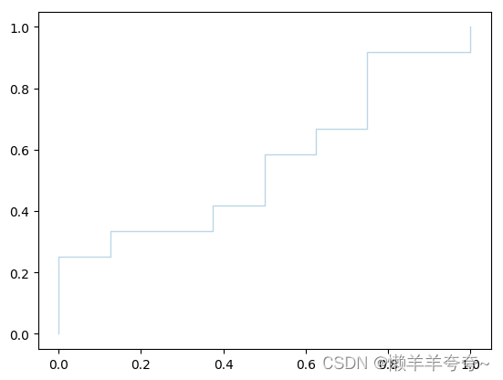
#ROC曲线

 

from sklearn.metrics import roc_curve, auc


tprs = []
aucs = []
mean_fpr = np.linspace(0, 1, 100)


probas_ = svc_clf.predict_proba(text_X)
fpr, tpr, thresholds = roc_curve(test_y, probas_[:, 1])
tprs.append(interp(mean_fpr, fpr, tpr))
tprs[-1][0] = 0.0
roc_auc = auc(fpr, tpr)
aucs.append(roc_auc)
plt.plot(fpr, tpr, lw=1, alpha=0.3,   label='ROC Curve (AUC = %0.2f)' % roc_auc)

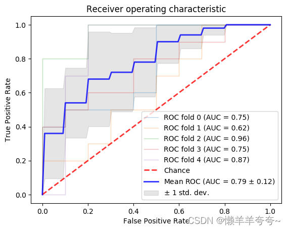
#交叉验证与ROC曲线
import numpy as np
from scipy import interp
import matplotlib.pyplot as plt
from sklearn import svm, datasets
from sklearn.metrics import roc_curve, auc
from sklearn.model_selection import StratifiedKFold


# 载入数据 只取第一类和第二类
iris = datasets.load_iris()
X = iris.data
y = iris.target
X, y = X[y != 2], y[y != 2]
n_samples, n_features = X.shape
# Add noisy features
random_state = np.random.RandomState(0)
X = np.c_[X, random_state.randn(n_samples, 200 * n_features)]

# 采用交叉验证的方式训练模型
cv = StratifiedKFold(n_splits=5)
classifier = svm.SVC(kernel='linear', probability=True,  random_state=random_state)


tprs = []
aucs = []
mean_fpr = np.linspace(0, 1, 100)


# 统计每次结果，并绘制相应的ROC曲线
i = 0
for train, test in cv.split(X, y):    
    probas_ = classifier.fit(X[train], y[train]).predict_proba(X[test])   
     # Compute ROC curve and area the curve
    fpr, tpr, thresholds = roc_curve(y[test], probas_[:, 1])    
    tprs.append(interp(mean_fpr, fpr, tpr))    
    tprs[-1][0] = 0.0    
    roc_auc = auc(fpr, tpr)    
    aucs.append(roc_auc)    
    plt.plot(fpr, tpr, lw=1, alpha=0.3,             
             label='ROC fold %d (AUC = %0.2f)' % (i, roc_auc))    
    i += 1
plt.plot([0, 1], [0, 1], linestyle='--', lw=2, color='r', 
         label='Chance', alpha=.8)

## 计算平均结果，绘制平均ROC曲线
mean_tpr = np.mean(tprs, axis=0)
mean_tpr[-1] = 1.0
mean_auc = auc(mean_fpr, mean_tpr)
std_auc = np.std(aucs)
plt.plot(mean_fpr, mean_tpr, color='b',
         label=r'Mean ROC (AUC = %0.2f $\pm$ %0.2f)' % (mean_auc, std_auc),
                  lw=2, alpha=.8)
## 将均值线上下一个标准差内的区域上色
std_tpr = np.std(tprs, axis=0)
tprs_upper = np.minimum(mean_tpr + std_tpr, 1)
tprs_lower = np.maximum(mean_tpr - std_tpr, 0)
plt.fill_between(mean_fpr, tprs_lower, tprs_upper, color='grey', alpha=.2,
                 label=r'$\pm$ 1 std. dev.')
plt.xlim([-0.05, 1.05])
plt.ylim([-0.05, 1.05])
plt.xlabel('False Positive Rate')
plt.ylabel('True Positive Rate')
plt.title('Receiver operating characteristic')
plt.legend(loc="lower right")
plt.show()