【Python高性能编程学习】第2讲 Profiling寻找性能瓶颈

最新推荐文章于 2025-03-13 07:29:54 发布

Domainmain

最新推荐文章于 2025-03-13 07:29:54 发布

阅读量1.2k

点赞数 19

分类专栏： Python高性能编程文章标签： python

本文链接：https://blog.csdn.net/qq_54501547/article/details/138318669

版权

Python高性能编程专栏收录该内容

7 篇文章

订阅专栏

参考：Micha Gorelick, Ian Ozsvald. High Performance Python: Practical Performant Programming for Humans. Second Edition

代码来源：GitHub - mynameisfiber/high_performance_python_2e: Code for the book "High Performance Python 2e" by Micha Gorelick and Ian Ozsvald with OReilly

前言说明

Profiling是一种重要的分析方法，可以帮助我们寻找到代码运行性能中的瓶颈（bottleneck），在这一篇笔记中我们将从CPU耗时和内存占用两个角度考察代码性能，主要目标有：

寻找运行较慢/占用较大的代码段
理解Python字节码，比较代码运行快慢
整合单元测试和性能测试
一些Profiling的策略和技巧

一、数据集准备

1.1 茱莉亚集（Julia Set）

Julia集是一个分形序列数据集，它通过迭代函数计算每一个像素点是否能够逃逸来决定该像素点的灰度，从而生成图像，如下图是一个Julia集的可视化结果：

我们以一个最简单的迭代函数为例：

$f(z)=z^2+c$

其中c是常数，z是复平面上像素点的表达式，即

$z=x+y*j$

其中j是虚数单位。那么对于复数z，它的模长|z|为：

$\left | z \right |=abs(z)=\sqrt{x^2+y^2}$

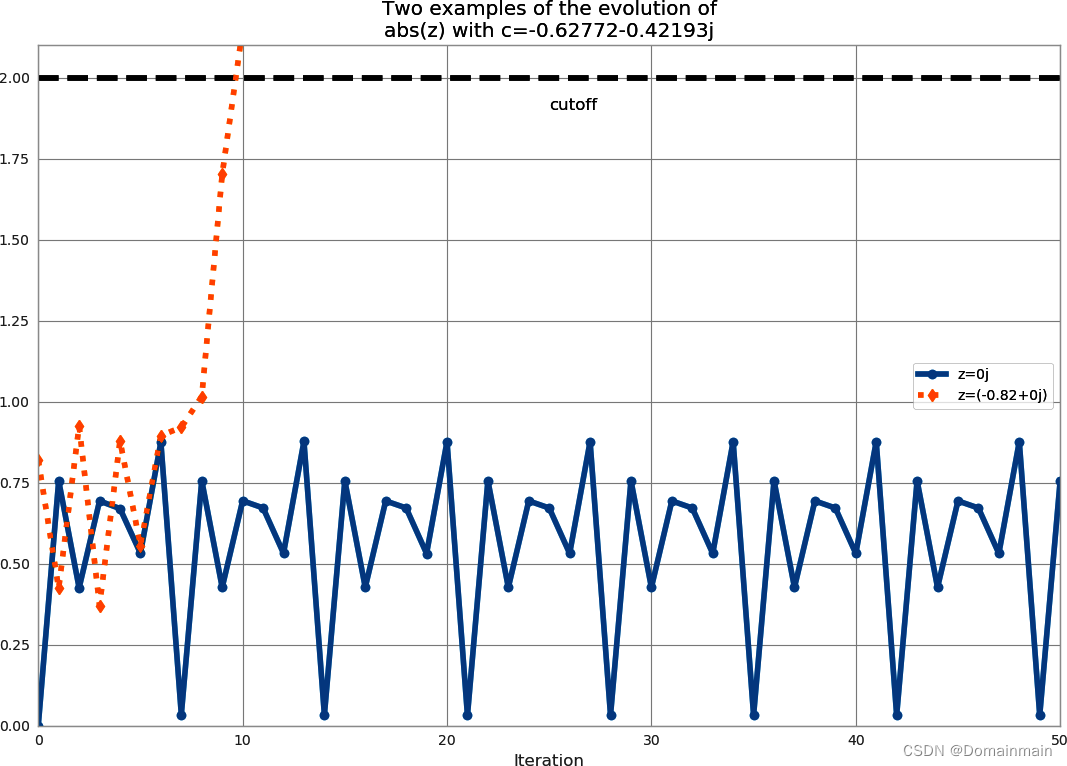
对于任意一个复数z，如果经历多次迭代，其模长仍然小于2，那么我们称这个复数属于囚犯集（Prisoner），反之如果经历有限次迭代就能使得其模长大于2，则称这个复数属于逃跑集（Escapee）。

如果我们把囚犯集的像素点设置为白色，把逃跑集的像素点设置为黑色，就形成了上面那张灰度图（当然上面那张图设置了阶梯颜色，但是不妨碍理解）。

我们使用Python代码再直观感受一下这个过程：

# 囚犯集
c = -0.62772-0.42193j
z = 0+0j
for n in range(12):
    z = z*z + c
    print(f"{n}: z={z: .5f}, abs(z)={abs(z):0.3f}, c={c: .5f}")
# 逃跑集
c = -0.62772-0.42193j
z = -0.82+0j
for n in range(12):
    z = z*z + c
    print(f"{n}: z={z: .5f}, abs(z)={abs(z):0.3f}, c={c: .5f}")

囚犯集的结果：

0: z=-0.62772-0.42193j, abs(z)=0.756, c=-0.62772-0.42193j
1: z=-0.41171+0.10778j, abs(z)=0.426, c=-0.62772-0.42193j 
2: z=-0.46983-0.51068j, abs(z)=0.694, c=-0.62772-0.42193j 
3: z=-0.66777+0.05793j, abs(z)=0.670, c=-0.62772-0.42193j 
4: z=-0.18516-0.49930j, abs(z)=0.533, c=-0.62772-0.42193j 
5: z=-0.84274-0.23703j, abs(z)=0.875, c=-0.62772-0.42193j 
6: z= 0.02630-0.02242j, abs(z)=0.035, c=-0.62772-0.42193j 
7: z=-0.62753-0.42311j, abs(z)=0.757, c=-0.62772-0.42193j 
8: z=-0.41295+0.10910j, abs(z)=0.427, c=-0.62772-0.42193j 
9: z=-0.46910-0.51203j, abs(z)=0.694, c=-0.62772-0.42193j 
10: z=-0.66985+0.05846j, abs(z)=0.672, c=-0.62772-0.42193j
11: z=-0.18244-0.50024j, abs(z)=0.532, c=-0.62772-0.42193j

逃跑集的结果：

0: z= 0.04468-0.42193j, abs(z)=0.424, c=-0.62772-0.42193j 
1: z=-0.80375-0.45963j, abs(z)=0.926, c=-0.62772-0.42193j 
2: z=-0.19297+0.31693j, abs(z)=0.371, c=-0.62772-0.42193j 
3: z=-0.69093-0.54425j, abs(z)=0.880, c=-0.62772-0.42193j
4: z=-0.44654+0.33014j, abs(z)=0.555, c=-0.62772-0.42193j
5: z=-0.53731-0.71677j, abs(z)=0.896, c=-0.62772-0.42193j
6: z=-0.85278+0.34833j, abs(z)=0.921, c=-0.62772-0.42193j
7: z=-0.02181-1.01603j, abs(z)=1.016, c=-0.62772-0.42193j
8: z=-1.65956-0.37760j, abs(z)=1.702, c=-0.62772-0.42193j
9: z= 1.98382+0.83138j, abs(z)=2.151, c=-0.62772-0.42193j
10: z= 2.61665+2.87669j, abs(z)=3.889, c=-0.62772-0.42193j
11: z=-2.05621+14.63263j, abs(z)=14.776, c=-0.62772-0.42193j

可以看到，0+0j在多次迭代后仍然没有突破2，但是-0.82+0j在第10次成功逃逸。下图同样展示了这样的结果。

1.2 茱莉亚集的产生代码

接下来我们要产生一个Julia集。第一步就是要确定像素点的范围和常数c的实部和虚部：

import time

x1, x2, y1, y2 = -1.8, 1.8, -1.8, 1.8
c_real, c_imag = -0.62772, -.42193

time包是用于计时的包。

接下来我们设置calc_pure_python函数，该函数接受参数desired_width和max_iterations，分别接收要划分的像素点的个数和最大迭代次数：

def calc_pure_python(desired_width, max_iterations):
    # 准备x,y坐标列表
    x_step = (x2 - x1) / desired_width
    y_step = (y1 - y2) / desired_width
    x = []
    y = []
    ycoord = y2
    while ycoord > y1:
        y.append(ycoord)
        ycoord += y_step
    xcoord = x1
    while xcoord < x2:
        x.append(xcoord)
        xcoord += x_step

    # 封装z和c
    zs = []
    cs = []
    for ycoord in y:
        for xcoord in x:
            zs.append(complex(xcoord, ycoord))
            cs.append(complex(c_real, c_imag))

    # 计算迭代次数
    print("Length of x:", len(x))
    print("Total elements:", len(zs))
    start_time = time.time()
    output = calculate_z_serial_purepython(max_iterations, zs, cs)
    end_time = time.time()
    secs = end_time - start_time
    print(calculate_z_serial_purepython.__name__ + " took", secs, "seconds")

    assert sum(output) == 33219980

在这其中，我们调用了calculate_z_serial_purepython函数，它会计算并返回每一个z的迭代次数。最后的断言语句（assert）是为了判断代码运行的正确性。

那么接下来就要编写calculate_z_serial_purepython函数了：

def calculate_z_serial_purepython(maxiter, zs, cs):
    output = [0] * len(zs)
    for i in range(len(zs)):
        n = 0
        z = zs[i]
        c = cs[i]
        while abs(z) < 2 and n < maxiter:
            z = z * z + c
            n += 1
        output[i] = n
    return output

这个函数就是Julia集最核心的部分，如果z是一个囚犯集，那么其返回的n值就是maxiter的值，否则是小于maxiter的值。

至此，我们就可以在主函数中去运行了。我们设置划分1000×1000个像素点，最大迭代次数为300次：

if __name__ == "__main__":
    calc_pure_python(desired_width=1000, max_iterations=300)

我们查看输出结果：

Length of x: 1000
Total elements: 1000000
calculate_z_serial_purepython took 6.397454023361206 seconds

由于每个机器实际运行的结果会不同，这个核心函数的耗时也会不同，这里的结果是我自己某一次实际运行的结果。

如果把图像绘制出来，应该是这样的：（包含画图的完整代码参见文章开头提供的源码地址）

二、Profiling方法的运用

2.1 耗时情况分析：time.time()

在上一部分我们就已经使用了time包中的time()函数记录了核心代码运行前后的时间点，二者相减就可以得到函数的耗时。这也是最简单、最直接地判断程序性能好坏的方式。

但是这样书写使得代码复用性和简洁性较差，因为我们必须要在函数内部插入计时器。是否可以把计时的功能单独编写完成，使得我们能够随时控制呢？这就可以通过Python装饰器实现：

from functools import wraps

def timefn(fn):
    @wraps(fn)
    def measure_time(*args, **kwargs):
        t1 = time.time()
        result = fn(*args, **kwargs)
        t2 = time.time()
        print(f"@timefn: {fn.__name__} took {t2 - t1} seconds")
        return result
    return measure_time


@timefn
def calculate_z_serial_purepython(maxiter, zs, cs):
    ...

我们定义了函数timefn()，参数为要计时的函数。
在timefn()内部定义一个函数measure_time()，由于calculate_z_serial_purepython()函数是带参的，所以给定*args和**kwargs。
我们在内部函数measure_time()中编写好计时的过程并返回函数运行结果。
使用functools.wraps方法和"@wraps(fn)"是为了使得被计时函数仍然保留自己原有的属性。
编写完成后，只需要在被计时函数的上一行写“@timefn”就可以完成计时，不需要计时则只需要注释掉这一行即可

运行结果示例：

Length of x: 1000
Total elements: 1000000
@timefn: calculate_z_serial_purepython took 8.55603575706482 seconds
calculate_z_serial_purepython took 8.55603575706482 seconds

当然，有时候装饰器和calc_pure_python自带的计时结果会有轻微的不同，这可能是由于函数调用或导入包的耗时差异，并不影响分析。

除了装饰器，还有别的方法也可以实现在不改变原函数结构的情况下完成计时，比如命令行工具timeit。其中-n表示运行的轮数，-r表示每一轮重复的次数，-s后面跟上"import python文件名"和“文件名.函数名()”，它会返回该脚本中指定函数运行n×r次后耗时最短的结果。

> python -m timeit -n 5 -r 1 -s "import julia1" \
"julia1.calc_pure_python(desired_width=1000, max_iterations=300)"
...
5 loops, best of 1: 7.88 sec per loop

当然，在IPython中可以使用%timeit完成，这里不再赘述。

2.2 函数调用分析：cProfile

除了看总体的时间，我们还可以对函数调用情况进行分析。cProfile是一个内置的标准库，它可以分析脚本中每一个函数的调用次数和运行用时，便于我们迅速锁定大量调用和运行缓慢的函数。

我们仍然以1.2中的代码为例，去掉画图的部分，文件命名为julia1_nopil.py，使用cProfile进行分析，其中-s cumulative表示对耗时进行累积：

> python -m cProfile -s cumulative julia1_nopil.py
Length of x: 1000
Total elements: 1000000
calculate_z_serial_purepython took 13.831141710281372 seconds
         36221995 function calls in 14.828 seconds

   Ordered by: cumulative time

   ncalls  tottime  percall  cumtime  percall filename:lineno(function)
        1    0.000    0.000   14.828   14.828 {built-in method builtins.exec}
        1    0.023    0.023   14.828   14.828 julia1_nopil.py:1(<module>)
        1    0.736    0.736   14.805   14.805 julia1_nopil.py:23(calc_pure_python)
        1    8.923    8.923   13.831   13.831 julia1_nopil.py:9(calculate_z_serial_purepython)
 34219980    4.908    0.000    4.908    0.000 {built-in method builtins.abs}
  2002000    0.230    0.000    0.230    0.000 {method 'append' of 'list' objects}
        1    0.007    0.007    0.007    0.007 {built-in method builtins.sum}
        3    0.001    0.000    0.001    0.000 {built-in method builtins.print}
        4    0.000    0.000    0.000    0.000 {built-in method builtins.len}
        2    0.000    0.000    0.000    0.000 {built-in method time.time}
        1    0.000    0.000    0.000    0.000 {method 'disable' of '_lsprof.Profiler' objects}

从返回的结果中我们可以看到：

总共有36221995次函数调用，总耗时14秒左右。
calc_pure_python和calculate_z_serial_purepython之间相差1秒，说明在调用除核心函数外的其他部分耗时为1秒。
calculate_z_serial_purepython调用1次，耗时9秒，其中abs的调用34219980次，非常耗时。但是有意思的是，每一次abs的调用是几乎不耗时的（percall≈0.000）。
append list这个操作调用2002000次，不难理解，因为zs和cs都是1000×1000的列表，x和y又都是长度为1000的列表，所以总和为2002000。
最后一行是lsprof，与cProfile有关，可忽略。

当然，如果你想要保存分析的结果，可以使用-o参数输出为.stats文件：

> python -m cProfile -o profile.stats julia1_nopil.py

之后使用pstats包进行读取：

import pstats
p = pstats.Stats("profile.stats") 
p.sort_stats("cumulative")
p.print_stats()     # 打印stats信息
p.print_callers()   # 打印每一个函数的调用者
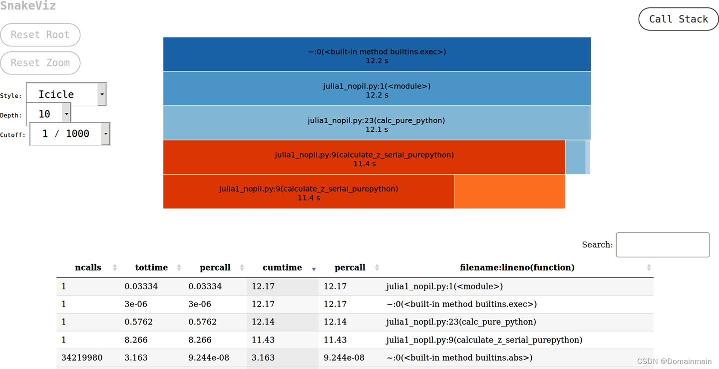
p.print_callees()   # 打印每一个函数的调用对象

最后，对于得到的profile.stats文件，可以使用SnakeViz进行可视化。首先使用python -m pip install snakeviz下载，之后运行snakeviz profile.stats，就能够在网页上交互式地展现结果：

2.3 逐行分析：line_profiler

如果找到了运行较慢的函数，我们一定想知道到底是哪一行耗时较长，这就要使用一个逐行分析工具line_profiler。使用之前应当通过python - m pip install line_profiler进行下载安装（如果下载连接超时估计需要科学上网或单独寻找安装包）。

使用line_profiler有两个要点：

需要在被分析函数的前面添加装饰器@profile
在命令行使用kernprof运行

@profile
def calculate_z_serial_purepython(maxiter, zs, cs):
    ...

@profile
def calc_pure_python(desired_width, max_iterations):
    ...

在命令行中，我们使用kernprof命令运行：

kernprof -l -v julia1_lineprofiler.py

其中-l表示line-by-line，-v表示可以直接显示运行日志。在命令行中，它会向我们返回装饰的这两个函数每一行的运行情况，同时也会生成.lprof文件，可以用line_profiler模块读取。

我们查看一下核心函数的运行情况：

Total time: 42.4309 s
File: julia1_lineprofiler.py
Function: calculate_z_serial_purepython at line 9

Line #      Hits         Time  Per Hit   % Time  Line Contents
==============================================================
     9                                           @profile
    10                                           def calculate_z_serial_purepython(maxiter, zs, cs):    
    11                                               """Calculate output list using Julia update rule"""
    12         1       1866.9   1866.9      0.0      output = [0] * len(zs)
    13   1000001     361804.3      0.4      0.9      for i in range(len(zs)):
    14   1000000     331477.0      0.3      0.8          n = 0
    15   1000000     384144.5      0.4      0.9          z = zs[i]
    16   1000000     359087.1      0.4      0.8          c = cs[i]
    17  34219980   17503470.4      0.5     41.3          while abs(z) < 2 and n < maxiter:
    18  33219980   12306459.0      0.4     29.0              z = z * z + c
    19  33219980   10777102.8      0.3     25.4              n += 1
    20   1000000     405509.9      0.4      1.0          output[i] = n
    21         1          7.8      7.8      0.0      return output

从返回的结果中我们可以看到：

整体耗时变长，因为我们对代码进行了逐行分析。
while循环条件判断耗时最长，甚至n+=1也占用了不小的时间（这是因为n+=1是一个复合操作，包含多个步骤）。

既然while循环非常耗时，那我们有必要深究while循环的语法逻辑。我们将while循环进行拆解：

@profile
def calculate_z_serial_purepython(maxiter, zs, cs):
    output = [0] * len(zs)
    for i in range(len(zs)):
        n = 0
        z = zs[i]
        c = cs[i]
        # 拆解
        while True:
            not_yet_escaped = abs(z) < 2
            iterations_left = n < maxiter
            if not_yet_escaped and iterations_left:
                z = z * z + c
                n += 1
            else:
                break
        output[i] = n
    return output

再运行kernprof：

kernprof -l -v julia1_lineprofiler2.py

Total time: 63.5656 s
File: julia1_lineprofiler2.py
Function: calculate_z_serial_purepython at line 9     

Line #      Hits         Time  Per Hit   % Time  Line Contents
==============================================================
     9                                           @profile
    10                                           def calculate_z_serial_purepython(maxiter, zs, cs):    
    11                                               """Calculate output list using Julia update rule"""
    12         1       2341.9   2341.9      0.0      output = [0] * len(zs)
    13   1000001     366001.5      0.4      0.6      for i in range(len(zs)):
    14   1000000     326636.3      0.3      0.5          n = 0
    15   1000000     385469.0      0.4      0.6          z = zs[i]
    16   1000000     353885.4      0.4      0.6          c = cs[i]
    17                                                   while True:
    18  34219980   16657884.4      0.5     26.2              not_yet_escaped = abs(z) < 2
    19  34219980   11730079.4      0.3     18.5              iterations_left = n < maxiter
    20  34219980   10534465.9      0.3     16.6              if not_yet_escaped and iterations_left:
    21  33219980   12221920.2      0.4     19.2                  z = z * z + c
    22  33219980   10603255.2      0.3     16.7                  n += 1
    23                                                       else:
    24                                                           break
    25   1000000     383659.0      0.4      0.6          output[i] = n
    26         1          9.9      9.9      0.0      return output

可以看到，while循环内部计算not_yet_escape和iterations_left这两个判断条件是最主要的耗时原因。事实上，这两个条件单独运行的结果是大有不同的：（取自书籍）

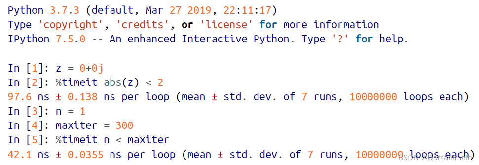
显然，由于要计算模长，abs(z)<2的耗时更长。
另外，从运算的结果来看，迭代总次数是33219980次，如果每一个像素点都属于囚犯集，即最坏的情况，迭代总次数应该为300*1000*1000=3千万次，也就是说，我们的结果仅仅只是最坏情况的10%，即abs(z)<2仅在10%的情况下为真。

综合这两种考虑，我们是否可以先让判断更快的n<maxiter放在前面，即：

while n < maxiter and abs(z) < 2

这样是否更快呢？

遗憾的是，Python 3.7对于多个并列条件没有位置顺序要求，即每一种写法造成的耗时几乎一致（Python 2.7则关乎条件的顺序），你可以用kernprof进行尝试。

虽然没有改进效果，但是这样的思考角度是值得学习的！

注：虽然说z=z*z+c耗时也同样多，但毕竟是不可能简化的步骤，所以不在考虑范围内。

2.4 内存占用分析：memory_profiler

除了时间分析，我们同样也关心内存的占用问题。可以从多个角度考虑，比如：

能否重写函数从而使用更少的RAM？
能否使用更多的RAM但是节省CPU的cycle数？

要完成内存占用分析，就要使用一个分析工具memory_profiler。使用之前应当通过python - m pip install memory_profiler进行下载安装（如果下载连接超时估计需要科学上网或单独寻找安装包）。

需要注意的是，内存占用分析是非常耗时的，如果使用完整的Julia集，可能会花费数小时。

memory_profiler的使用方法与cProfile类似，但是仍然要在函数面前添加@profile：

python -m memory_profiler julia1_memoryprofiler.py

这里我们直接截取书籍上的一部分结果：

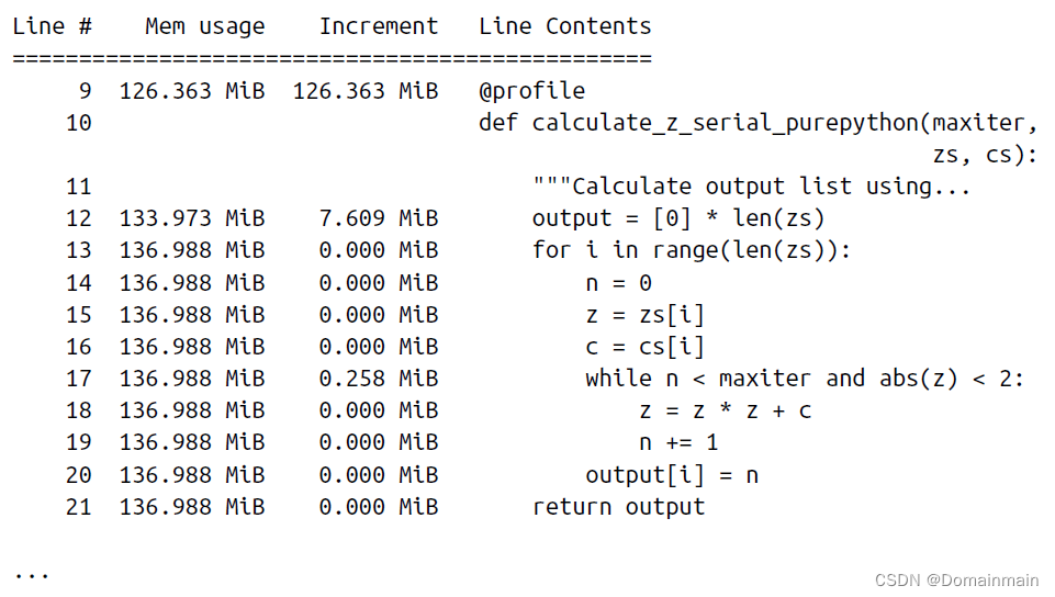
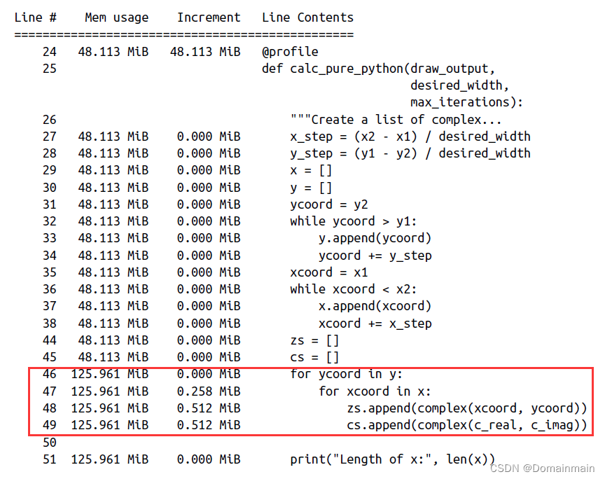
从结果中我们可以看到：

output列表创建使得RAM增加7MB，当然这并不是说output列表占据7MB，而是在为output列表分配空间的过程增加了7MB的使用空间。
zs和cs列表的占用量很大。
Increment列和Mem usage列似乎不匹配，这是一个小bug，但是以Mem usage为主来进行分析即可。

一般来说，内存分配往往会过度，并且由于垃圾回收机制并不是及时的，所以这种内存占用分析不会像CPU使用分析那么精确，我们在使用这个工具时一般从增长趋势等感性的认识出发，不要过多纠结数值的准确性。

同样地，memory_profiler包含可视化工具mprof，可以对内存分析可视化：

mprof run julia1_memoryprofiler.py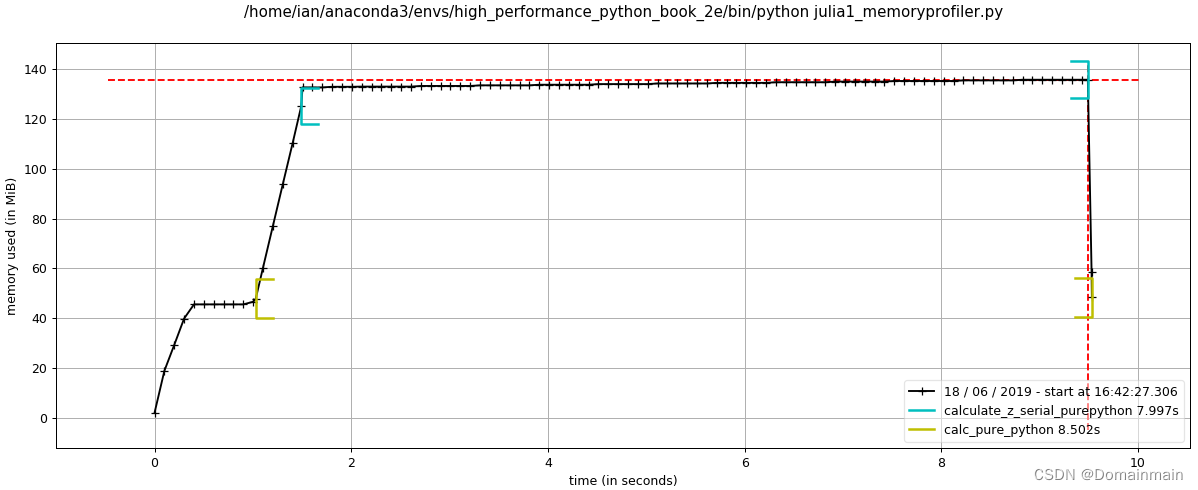

如果我们把zs和cs改成动态的变量而不是存储列表，你会发现内存占用一下子就减轻了：

@profile
def calculate_z_serial_purepython(maxiter, x, y):
    output = []
    for ycoord in y:
        for xcoord in x:
            z = complex(xcoord, ycoord)
            c = complex(c_real, c_imag)
            n = 0
            while n < maxiter and abs(z) < 2:
                z = z * z + c
                n += 1
            output.append(n)
    return output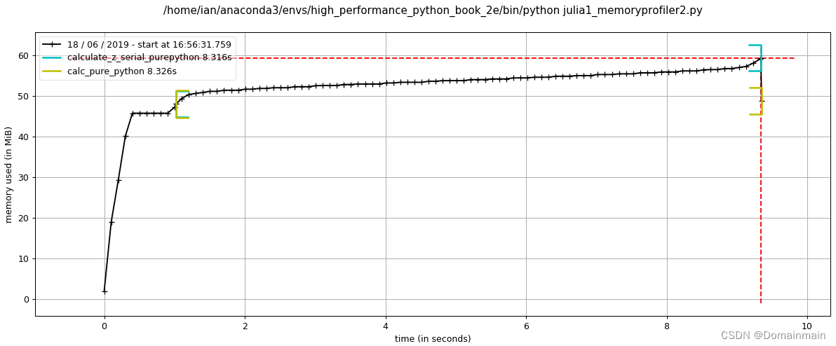

2.5 运行过程监测：PySpy

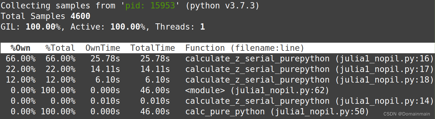
最后，如果一个Python脚本运行较慢或是已经投入使用的代码，由于无法随时重新运行代码，就可以在它运行的过程中进行监视，从而返回一个像top命令的结果。一般在Linux上运行。

首先使用ps -A -o pid,rss,cmd | ack python找到程序对应的pid，之后使用py-spy --pid xxxx来运行，返回结果示意：

如果你使用--flame参数，则可以可视化这个结果：

py-spy --flame profile.svg --pid xxxx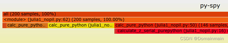

三、Profiling的其他要点和技巧

3.1 显式函数和内置函数的效率差异

除了从耗时和内存占用的角度来分析，我们还可以从函数效率上分析。我们知道Python中有很多内置函数，这些函数往往比我们自己写的函数要更高效。比如以下两种求和的函数：

def fn_expressive(upper=1000000):
    total = 0
    for n in range(upper):
        total += n
    return total

def fn_terse(upper=1000000):
    return sum(range(upper))

我们使用%tmeit来测试一下：

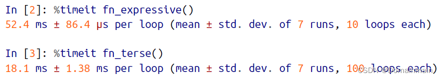
的确，后一种函数的效率更高。这是为什么呢？

我们使用内置模块dis来分析两个函数的字节码：

import dis
dis.dis(fn_expressive)
print("---------------")
dis.dis(fn_terse)

  2           0 LOAD_CONST               1 (0)
              2 STORE_FAST               1 (total)

  3           4 LOAD_GLOBAL              0 (range)
              6 LOAD_FAST                0 (upper)
              8 CALL_FUNCTION            1        
             10 GET_ITER
        >>   12 FOR_ITER                12 (to 26)
             14 STORE_FAST               2 (n)    

  4          16 LOAD_FAST                1 (total)
             18 LOAD_FAST                2 (n)
             20 INPLACE_ADD
             22 STORE_FAST               1 (total)
             24 JUMP_ABSOLUTE           12

  5     >>   26 LOAD_FAST                1 (total)
             28 RETURN_VALUE
---------------
  8           0 LOAD_GLOBAL              0 (sum)
              2 LOAD_GLOBAL              1 (range)
              4 LOAD_FAST                0 (upper)
              6 CALL_FUNCTION            1
              8 CALL_FUNCTION            1
             10 RETURN_VALUE

可以看到，后者使用sum和range两个函数采取了优化后的列表推导，使得代码效率更高，而前者要定义多个变量和迭代器，代码变得低效。

如果Python中有高效的内置函数，请考虑是否可以使用。

3.2 No-op @profile：单元测试与Profiling的整合

单元测试是检查代码正确性的重要手段，但是如果使用@profile装饰器会报错，因为这是没有声明或引入的方法：

import time

def test_some_fn():
    """Check basic behaviours for our function"""
    assert some_fn(2) == 4
    assert some_fn(1) == 1
    assert some_fn(-1) == 1

@profile
def some_fn(useful_input):
    time.sleep(1) 
    return useful_input ** 2


if __name__ == "__main__":
    print(f"Example call `some_fn(2)` == {some_fn(2)}")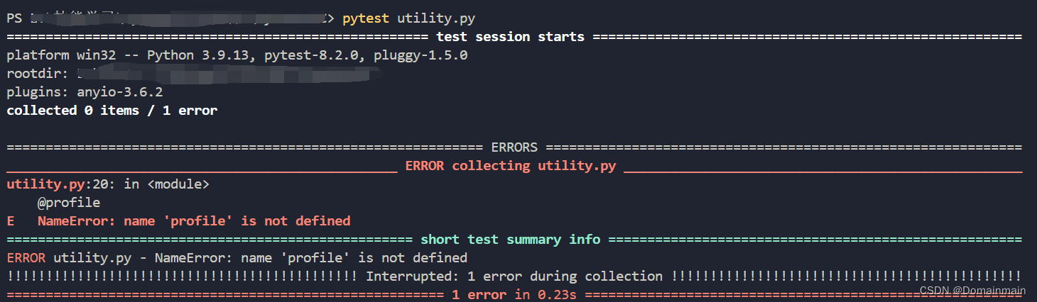

如果要整合单元测试和Profiling，就要增加装饰器的闭包写法：

import time

def test_some_fn():
    """Check basic behaviours for our function"""
    assert some_fn(2) == 4
    assert some_fn(1) == 1
    assert some_fn(-1) == 1

if 'line_profiler' not in dir() and 'profile' not in dir():
    def profile(func):
        def inner(*args, **kwargs):
            return func(*args, **kwargs)
        return inner

@profile
def some_fn(useful_input):
    time.sleep(1) 
    return useful_input ** 2


if __name__ == "__main__":
    print(f"Example call `some_fn(2)` == {some_fn(2)}")

这样就能正常运行了。