有限元分析中的经典前处理（映射法和扫略法）

1. 映射法

import numpy as np
import matplotlib.pyplot as plt
'''
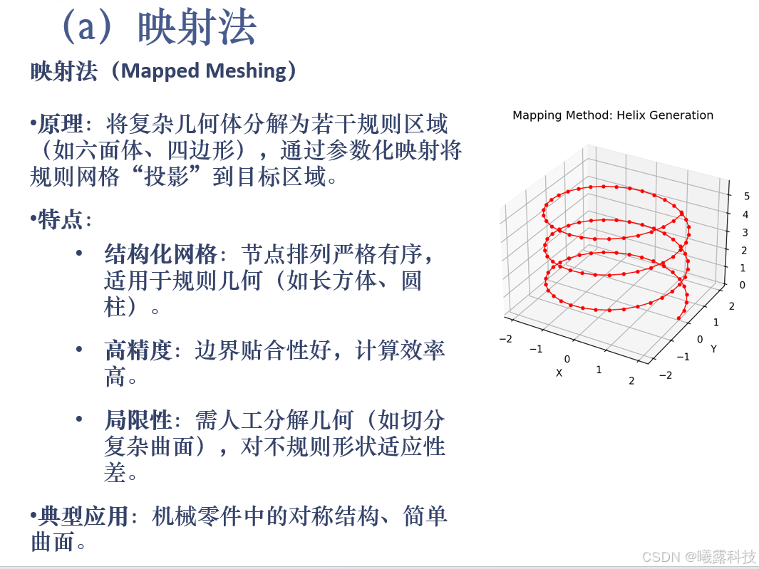
映射法（Mapping Method）
原理：将参数空间的一维直线映射到物理空间的螺旋线。
'''

# 参数设置
R = 2.0       # 螺旋线半径
k = 0.3       # 螺距参数（z轴每弧度增量）
n_turns = 3   # 圈数
n_points = 100  # 离散点数量

# 参数设置
t = np.linspace(0, 1, n_points)  # 归一化参数

# 将t映射到螺旋线参数θ
theta_mapped = t * 2 * np.pi * n_turns  # 映射到角度范围

# 计算坐标
x_mapped = R * np.cos(theta_mapped)
y_mapped = R * np.sin(theta_mapped)
z_mapped = k * theta_mapped

# 可视化
fig = plt.figure()
ax = fig.add_subplot(111, projection='3d')
ax.plot(x_mapped, y_mapped, z_mapped, 'r-o', markersize=3, linewidth=1)
ax.set_xlabel('X')
ax.set_ylabel('Y')
ax.set_zlabel('Z')
plt.title('Mapping Method: Helix Generation')
plt.show()

2. 扫略法

import numpy as np
import matplotlib.pyplot as plt
from mpl_toolkits.mplot3d import Axes3D
'''
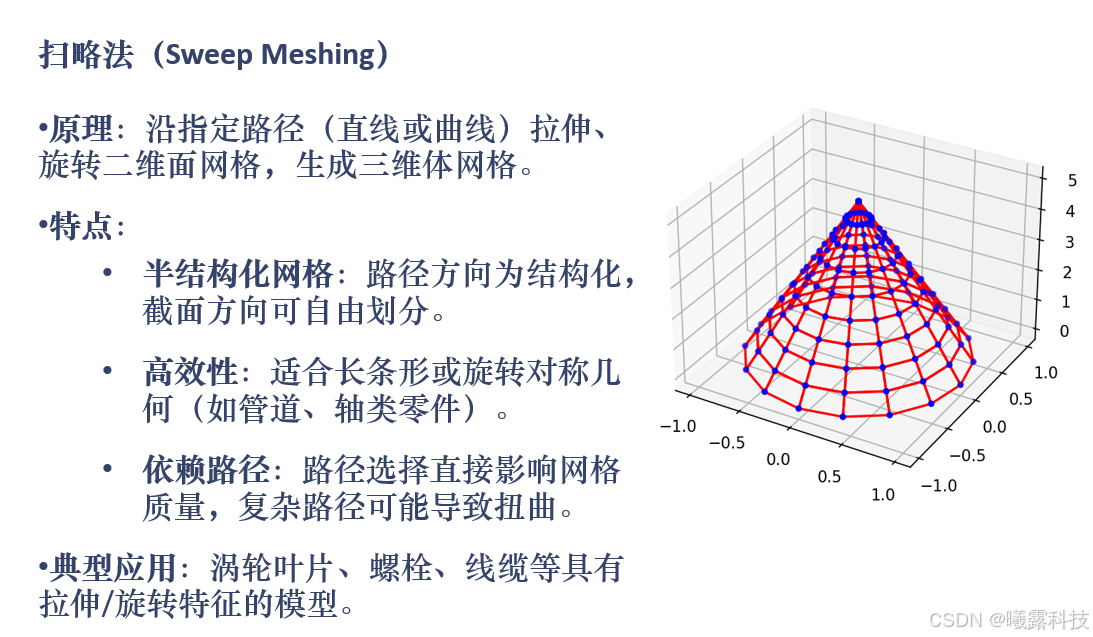
扫略法
'''
def sweep_method_cone(R=1.0, H=5.0, n_circle=8, n_height=5):
    """
    扫略法生成圆锥体网格
    公式：x = R*(1 - z/H)*cosθ, y = R*(1 - z/H)*sinθ, z = h (θ∈[0,2π], h∈[0,H])
    """
    # 生成节点
    theta = np.linspace(0, 2 * np.pi, n_circle, endpoint=False)
    z_values = np.linspace(0, H, n_height)  # 修正了linspace参数
    nodes = []
    for z in z_values:
        current_R = R * (1 - z / H)  # 半径随高度线性减小
        for t in theta:
            x = current_R * np.cos(t)
            y = current_R * np.sin(t)
            nodes.append([x, y, z])
    nodes = np.array(nodes)

    # 生成四边形单元（扫略特征）
    elements = []
    for i in range(n_height - 1):
        for j in range(n_circle):
            n1 = i * n_circle + j
            n2 = i * n_circle + (j + 1) % n_circle
            n3 = (i + 1) * n_circle + (j + 1) % n_circle
            n4 = (i + 1) * n_circle + j
            elements.append([n1, n2, n3, n4])

    return nodes, np.array(elements)

# 示例使用和可视化
nodes, elements = sweep_method_cone(R=1.0, H=5.0, n_circle=16, n_height=10)

fig = plt.figure()
ax = fig.add_subplot(111, projection='3d')
ax.scatter(nodes[:,0], nodes[:,1], nodes[:,2], c='b', s=10)

# 绘制四边形单元
for elem in elements:
    # 连接四边形顶点
    for i in range(4):
        start = nodes[elem[i]]
        end = nodes[elem[(i+1)%4]]
        ax.plot([start[0], end[0]], [start[1], end[1]], [start[2], end[2]], 'r-')

plt.show()

参考资料

【1】S.H. Lo, Finite Element Mesh Generation, CRC PressTaylor & Francis USA, 2015

【2】阿里云-常用的有限元网格生成方法