


本文介绍——
1.如何定义高斯传感器频率响应:当响应具有高斯形状时,如何表达探测器的频率响应(例如:压电超声换能器),基于均质传播介质示例;
2.模拟函数的比较:介绍模拟函数"kspaceFirstOrder2D"和"kspaceecondorder"之间的简短比较。基于均匀传播介质和使用二进制传感器示例;
3.如何设置初始压力梯度。
注:这三个示例本人理解的不太好,一些内容是官方英文注释的机翻,还请辩证性阅读。
有兴趣的同好可以加企鹅群交流:937503xxx(有意向的同好私聊或评论加群,新群,目前群内仅5人),任何科研相关问题都可以在群内交流,平常一起聊聊天、分享日常也是没问题的,欢迎~
目录
一、定义高斯传感器频率响应
1.1 定义传感器频率响应
% define the frequency response of the sensor elements
center_freq = 3e6;      % [Hz]
bandwidth = 80;         % [%]
sensor.frequency_response = [center_freq, bandwidth];
center_freq = 3e6; % [Hz] 中心频率
bandwidth = 80; % [%] 带宽百分比
sensor.frequency_response = [center_freq, bandwidth];
% 利用传感器输入结构的"frequency_response"字段来分配传感器的频率响应。
% 有两个参数:(1)中心频率,用于频率响应的带宽。
% (2)换能器带宽,定义为百分比,控制滤波器的半最大值全宽度(FWHM),其中FWHM = %带宽*中心频率(如图)。
% 当定义了"sensor.frequency_response"的输入时,在仿真完成后,
% 通过使用"gaussianFilter"将傅里叶变换后的信号乘以零相位高斯窗口,在仿真函数中应用高斯滤波器。
% 注意,当返回传感器数据时,也可以通过显式调用"gaussianFilter"轻松地应用相同的过滤器。

1.2 运行模拟与可视化
% re-run the simulation
sensor_data_filtered = kspaceFirstOrder2D(kgrid, medium, source, sensor);

% calculate the frequency spectrum at the first sensor element
[~, sensor_data_as] = spect(sensor_data(1, :), 1/kgrid.dt);
[f, sensor_data_filtered_as] = spect(sensor_data_filtered(1, :), 1/kgrid.dt);
注:上述只给出新增的代码程序,其他常规定义未给出
% 重新运行模拟
sensor_data_filtered = kspaceFirstOrder2D(kgrid, medium, source, sensor);
% 计算第一个传感器元件的频谱
[~, sensor_data_as] = spect(sensor_data(1, :), 1/kgrid.dt);
[f, sensor_data_filtered_as] = spect(sensor_data_filtered(1, :), 1/kgrid.dt);
% "spect":计算单面振幅和相位谱
% [f, func_as, func_ps] = spect(func, Fs, ...)
% func:要分析的信号,Fs:采样频率[Hz]
% f:频率数组,func_as:单面振幅谱,func_ps:单面相位谱
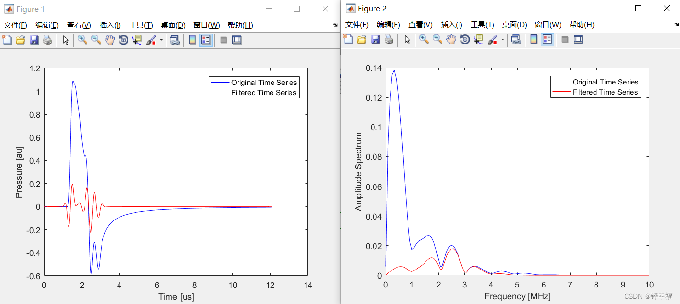
% 在定义与没定义"sensor.frequency_response"字段的模拟中,
% 计算第一个传感器位置记录的时间序列如下,并给出了相应的振幅谱。
% 低频信息的去除对信号幅值有显著影响。
% "sensor_data"与"sensor_data_as"为没有定义高斯传感器频率响应时;
% "sensor_data_filtered"与"sensor_data_filtered_as"为定义了高斯传感器频率响应。
% plot the simulated sensor data at the first sensor element
figure;
[t_sc, scale, prefix] = scaleSI(max(kgrid.t_array(:)));
plot(scale * kgrid.t_array, sensor_data(1, :), 'b-', ...
     scale * kgrid.t_array, sensor_data_filtered(1, :), 'r-');
ylabel('Pressure [au]');
xlabel(['Time [' prefix 's]']);
legend('Original Time Series', 'Filtered Time Series');

% plot the amplitude spectrum
figure;
[f_sc, scale, prefix] = scaleSI(max(f(:)));
plot(scale * f, sensor_data_as, 'b-', ...
     scale * f, sensor_data_filtered_as, 'r-');
ylabel('Amplitude Spectrum');
xlabel(['Frequency [' prefix 'Hz]']);
legend('Original Time Series', 'Filtered Time Series');
set(gca, 'XLim', [0 10]);
% 在第一传感器元件处绘制模拟传感器数据,随时间变化的压力图(如下左图)
figure;
[t_sc, scale, prefix] = scaleSI(max(kgrid.t_array(:)));
% 注释:max(kgrid.t_array(:))=1.2060*10^(-5);t_sc=0.12,scale=10^6,prefix='u'
plot(scale * kgrid.t_array, sensor_data(1, :), 'b-', ...
scale * kgrid.t_array, sensor_data_filtered(1, :), 'r-');
ylabel('Pressure [au]'); % 注:Pressure [au] 表示为什么物理量与单位,本人尚且不知,此坑留下0.q
xlabel(['Time [' prefix 's]']);
legend('Original Time Series', 'Filtered Time Series');
% "legend":向图形添加图例:“原始时间序列”,“过滤时间序列”
% 绘制振幅谱,随频率变化的振幅图(如下右图)
figure;
[f_sc, scale, prefix] = scaleSI(max(f(:)));
% 注释:max(f(:))=25000000;f_sc=25,scale=10^6,prefix='M'
% 下面程序同上,略
% 蓝色线条为没有定义高斯传感器频率响应时,红色线条为定义了高斯传感器频率响应。
二、模拟函数的比较
2.1 关于模拟函数
在前面的例子中,声学模拟都是使用"kspaceFirstOrder2D"进行的。
该函数基于粒子速度、声密度和声压的顺序计算,使用三个耦合的一阶偏微分方程(质量守恒、动量守恒和压力-密度关系)。
对于均匀介质,这些方程也可以合并成一个二阶声波方程,用格林函数法求解。
ps.格林函数:是一种用来解有初始条件或边界条件的非齐次微分方程的函数。
函数"kspaceSecondOrder"是格林函数解的有效数值实现,专门用于初值问题。
对于均匀介质,这两种方法给出相同的结果。
与"kspaceFirstOrder2D"相比,函数"kspaceSecondOrder"具有更高的计算效率,并且时间步长可以任意大(因为解是精确的)。
它还允许定义初始压力和初始压力梯度(参见设置初始压力梯度示例)。
幂律吸收也被更精确地编码(参见幂律吸收的建模示例)。
然而,"kspaceecondorder"的功能比它的一阶对应物(kspaceFirstOrder1D、kspaceFirstOrder2D和kspaceFirstOrder3D)稍微少一些。
例如:它只支持均匀介质和二进制传感器,不支持时变源或全范围的可视化选项。
二阶代码没有实现吸收边界层(可参见控制吸收边界层示例:Controlling The Absorbing Boundary Layer Example,了解"kspaceFirstOrder2D"中使用的PML(完美匹配层)的更多细节)。
相反,为了延迟波包裹的出现,它扩展了计算网格的大小。
虽然这降低了计算效率,但它可以保持解决方案的准确性。
通过将可选输入参数"ExpandGrid"设置为"true"来控制网格扩展。
注意,如果模拟时间比波通过网格扩展传播所需的时间长,仍然会出现包裹波。
2.2 运行模拟
example_number = 1;
% 1: non-absorbing medium, no absorbing boundary layer
% 2: non-absorbing medium, using PML and ExpandGrid
% 3: absorbing medium, no absorbing boundary layer
% 4: absorbing medium, using PML and ExpandGrid

% define the properties of the propagation medium
medium.sound_speed = 1500;  % [m/s]
if example_number > 2
    medium.alpha_power = 1.5;   % [dB/(MHz^y cm)]
    medium.alpha_coeff = 0.75;  % [dB/(MHz^y cm)]
end

% define a centered circular sensor pushed right to the edge of the grid
sensor_radius = 6.3e-3;   % [m]
num_sensor_points = 50;
sensor.mask = makeCartCircle(sensor_radius, num_sensor_points);

% convert the cartesian sensor mask to a binary sensor mask
sensor.mask = cart2grid(kgrid, sensor.mask);

if example_number == 1  || example_number == 3

    % run the simulation using the first order code
    sensor_data_first_order = kspaceFirstOrder2D(kgrid, medium, source, sensor, 'PMLAlpha', 0);

    % run the simulation using the second order code
    sensor_data_second_order = kspaceSecondOrder(kgrid, medium, source, sensor, 'ExpandGrid', false);

elseif example_number == 2  || example_number == 4  % using PML and ExpandGrid

    % run the simulation using the first order code
    sensor_data_first_order = kspaceFirstOrder2D(kgrid, medium, source, sensor, 'PMLInside', false);

    % run the simulation using the second order code
    sensor_data_second_order = kspaceSecondOrder(kgrid, medium, source, sensor, 'ExpandGrid', true);

end
注:上述只给出新增的代码程序,其他常规定义未给出
example_number = 1;
% 1:非吸收介质,无吸收边界层
% 2:非吸收介质,使用PML和ExpandGrid
% 3:吸收介质,无吸收边界层
% 4:吸收介质,使用PML和ExpandGrid
% 半径设置为6.3[mm],传感器紧贴网格的边缘(因为网格大小为[-6.4mm, 6.4mm])
sensor_radius = 6.3e-3; % [m]
num_sensor_points = 50;
sensor.mask = makeCartCircle(sensor_radius, num_sensor_points);
% 将笛卡尔传感器转换为二进制传感器
sensor.mask = cart2grid(kgrid, sensor.mask);
% 函数"kspaceSecondOrder"(用于所有维度)采用与一阶模拟函数相同的输入结构。
% 例如,要运行均匀传播介质示例,首先使用"cart2grid"将笛卡尔传感器掩码转换为二进制传感器掩码,
% 然后调用"kspaceSecondOrder"并将"ExpandGrid"设置为"true"。
if example_number == 1 || example_number == 3 % 1、3为无吸收边界层
sensor_data_first_order = kspaceFirstOrder2D(kgrid, medium, source, sensor, 'PMLAlpha', 0); % 一阶
sensor_data_second_order = kspaceSecondOrder(kgrid, medium, source, sensor, 'ExpandGrid', false); % 二阶
elseif example_number == 2 || example_number == 4 %2、4为使用PML和ExpandGrid
sensor_data_first_order = kspaceFirstOrder2D(kgrid, medium, source, sensor, 'PMLInside', false); % 一阶
sensor_data_second_order = kspaceSecondOrder(kgrid, medium, source, sensor, 'ExpandGrid', true); % 二阶
end
2.3 可视化
% plot a single time series
figure;
[t_sc, t_scale, t_prefix] = scaleSI(kgrid.t_array(end));
subplot(2, 1, 1);
plot(kgrid.t_array*t_scale, sensor_data_second_order(1, :), 'k-', ...
     kgrid.t_array*t_scale, sensor_data_first_order(1, :), 'bx'); %'bx':蓝色的x
set(gca, 'YLim', [-1, 1.5]);
xlabel(['Time [' t_prefix 's]']);
ylabel('Pressure [au]');
legend('kspaceSecondOrder', 'kspaceFirstOrder2D', 'Location', 'NorthWest');
title('Recorded Signals');

subplot(2, 1, 2);
plot(kgrid.t_array*t_scale, sensor_data_second_order(1, :) - sensor_data_first_order(1, :), 'k-');
xlabel(['Time [' t_prefix 's]']);
ylabel('Pressure [au]');
title('Difference In Recorded Signals');
第一幅图绘制单个时间序列,记录信号;第二幅图记录信号之间的差异
%'bx':将线条绘制为蓝色的x(如图)
legend('kspaceSecondOrder', 'kspaceFirstOrder2D', 'Location', 'NorthWest');
% 'Location', 'NorthWest':将图例设置在左上角(西北方)。
% 在不吸收介质和不补偿包波的情况下,两种模拟函数在机器精度上是一致的。
% 左图是在第一个传感器位置记录的信号及其之间的差异(设置example_number = 1)。
% 当介质被吸收并使用完全匹配层来减轻波包裹时,使用"kspaceFirstOrder2D"计算的数值结果有很小的误差。
% 这种误差很大程度上是由于幂律吸收项的计算造成的(参见幂律吸收的建模示例:Modelling Power Law Absorption Example)。
% 右图是在第一个传感器位置记录的信号及其之间的差异(设置example_number = 4)。


三、设置初始压力梯度
3.1 定义声源属性
% set plot_frames to true to produce the plots given in the documentation
% or false to visualise the propagation of the pressure field
plot_frames = true;
if plot_frames

    % calculate and plot the pressure at a particular value of t
    Nt = 2;
    dt = 1e-6;  % [s]
    kgrid.setTime(Nt, dt);

else

    % calculate the plot the progression of the pressure field with t
    dt = 5e-9;  % [s]
    Nt = round(5e-6 / dt);
    kgrid.setTime(Nt, dt);

end

% create source distribution using makeDisc
disc_magnitude = 4; % [Pa]
disc_x_pos = 25;    % [grid points]
disc_y_pos = 40;    % [grid points]
disc_radius = 4;    % [grid points]
disc_1 = disc_magnitude * makeDisc(Nx, Ny, disc_x_pos, disc_y_pos, disc_radius);

disc_magnitude = 3; % [Pa]
disc_x_pos = 40;    % [grid points]
disc_y_pos = 25;    % [grid points]
disc_radius = 3;    % [grid points]
disc_2 = disc_magnitude * makeDisc(Nx, Ny, disc_x_pos, disc_y_pos, disc_radius);

source_distribution = disc_1 + disc_2;

% define a single sensor point
sensor.mask = zeros(Nx, Ny);
sensor.mask(Nx/2, Ny/2) = 1;

% define the input arguments
input_args = {'PlotFrames', plot_frames, 'MeshPlot', true, ...
    'PlotScale', [0 3], 'ExpandGrid', true};
注:上述只给出新增的代码程序,其他常规定义未给出
% 将plot_frames设置为true以生成文档中给出的图形,或将plot_frames设置为false以可视化压力场的传播。
% 使用"makeDisc"创建两个不同直径的小磁盘的初始声源分布
input_args = {'PlotFrames', plot_frames, 'MeshPlot', true, ...
'PlotScale', [0 3], 'ExpandGrid', true};
% 选输入"MeshPlot"设置为"true",以允许压力场的3D可视化。
% 如果"PlotFrames"设置为"true",则单个帧将在新图形中生成。
% 使用"PlotScale"设置图像缩放,使用"ExpandGrid"设置为"true"来控制网格扩展。
3.2 可视化
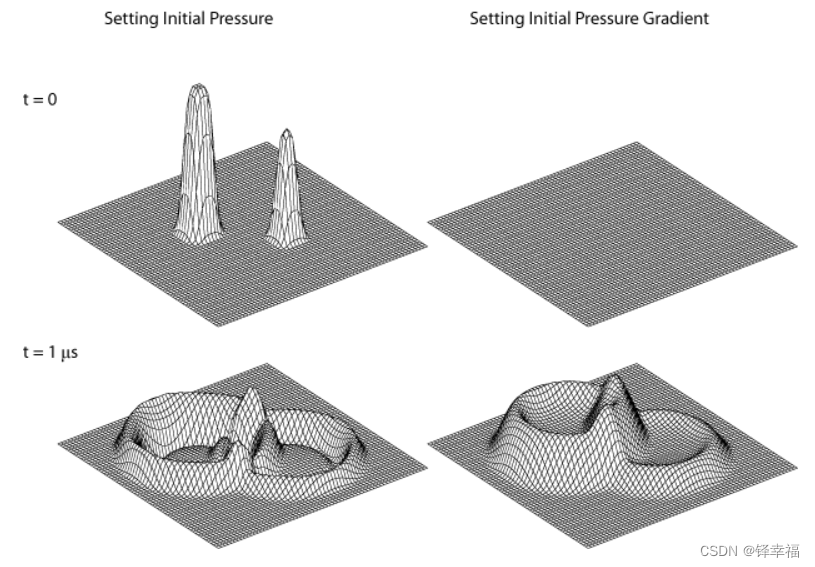
函数"kspaceSecondOrder"允许定义初始压力及其时间梯度的初始条件。
初始条件定义为与计算网格大小相同的数值矩阵。
初始压力赋值给"source_p0",初始压力梯度赋值给"source.dp0dt"
% assign the source distribution to the initial pressure
source.p0 = source_distribution;
kspaceSecondOrder(kgrid, medium, source, sensor, input_args{:});

% assign the source distribution to the initial pressure gradient
source = rmfield(source, 'p0');
source.dp0dt = 5e6 * source_distribution;
kspaceSecondOrder(kgrid, medium, source, sensor, input_args{:});

% assign the source distribution to both the initial pressure and the
% initial pressure gradient
source.p0 = source_distribution;
kspaceSecondOrder(kgrid, medium, source, sensor, input_args{:});
% 将源分布分配给初始压力
source.p0 = source_distribution;
kspaceSecondOrder(kgrid, medium, source, sensor, input_args{:});
% 将源分布分配给初始压力梯度
source = rmfield(source, 'p0');
% "rmfield":从结构中删除字段
% 从"source"中删除"p0",即从"source"中删除刚刚分配的初始压力
source.dp0dt = 5e6 * source_distribution;
kspaceSecondOrder(kgrid, medium, source, sensor, input_args{:});
% 将源分布分配给初始压力和初始压力梯度
source.p0 = source_distribution;
% 重新在"source"加入初始压力,此时的"source"同时有初始压力和初始压力梯度
kspaceSecondOrder(kgrid, medium, source, sensor, input_args{:});
下面是两个不同 t 值下的压力场图:


 9837
9837


 被折叠的 条评论
为什么被折叠?
被折叠的 条评论
为什么被折叠?
 到【灌水乐园】发言


