循环神经网络（RNN）_6

牛+马=我

已于 2022-04-09 18:17:20 修改

阅读量1k

点赞数

分类专栏：深度学习与神经网络文章标签： python tensorflow keras 循环神经网络神经网络

于 2022-04-09 14:33:01 首次发布

本文链接：https://blog.csdn.net/qq_57780419/article/details/124053430

版权

深度学习与神经网络专栏收录该内容

7 篇文章 1 订阅

订阅专栏

用RNN实现连续数据的预测（以股票预测为例）

循环核：参数时间共享，循环层提取时间信息

在这里插入图片描述
当记忆体个数被指定，输入Xt,输出Yt的维度被指定
Wxh，Whh，Why的维度也被指定了
记忆体存储有每个时刻的状态信息：ht

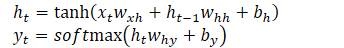
前向传播：记忆体内存储的状态信息ht，在每个时刻都被刷新，三个参数Wxh,Whh,Why自始至终都是不变的
反向传播：三个参数矩阵Wxh，Whh，Why被梯度下降法更新

循环核按时间步展开：就是按时间轴的方向展开

在这里插入图片描述

这整个时间轴是一个前向传播，Wxh，Whh，Why是不变的
反向传播的时候才变
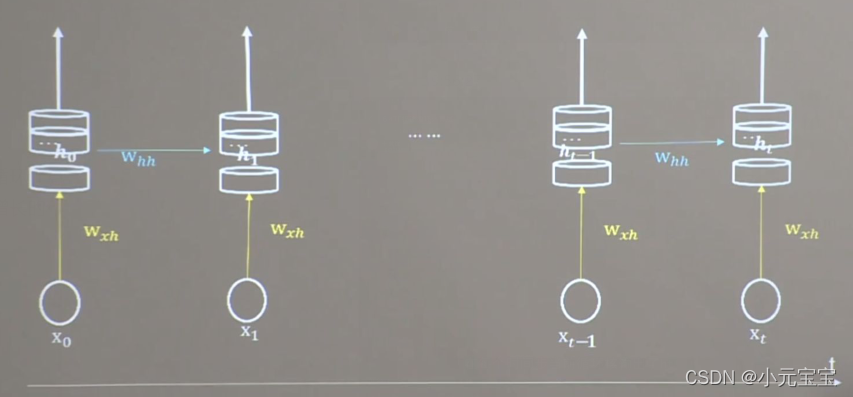
循环神经网络：借助循环核提取时间特征后，送入全连接神经网络

循环计算层：每个循环核构成一层循环计算层

循环计算层的层数是向着输出方向增长的
在这里插入图片描述

TF描述循环计算层：

tf.keras.layers.SimpleRNN(循环核中记忆体的个数，activation=‘激活函数’，return_sequences=是否每个时刻输出到ht到下一层)

activation=‘激活函数’：表示使用什么激活函数计算ht，如果不写，默认tanh
return_sequences=True：表示各时间步输出ht到下一层
return_sequences=False：表示仅在最后时间步输出ht（默认）
return_sequences=True：
在这里插入图片描述
return_sequences=False：

一般最后一层的循环核用False，中间层的循环核用True：表示每个时间步都把参数输出到下一层，仅在最后时间步输出ht
如下图：

如tf.keras.layers.SimpleRNN(3,return_sequences=True)

要求送入RNN的数据是三维的，即x_train是三维的：
[送入样本数，循环核时间展开步数，每个时间步输入特征个数]
在这里插入图片描述
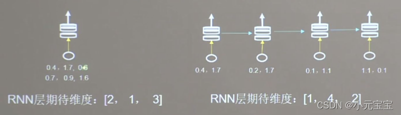
如上图的第一个图：以关送入RNN2组数据，每组数据经过1个时间步即可输出结果，每个时间步送入3个数值。所以是[2,1,3]

输入一个字母进行RNN预测

问题：

用RNN实现输入一个字母，预测出下一个字母（字母使用独热编码）：
输入a，预测出b
输入b，预测出c
输入c，预测出d
输入d，预测出e
输入e，预测出a

分析：

1.import
2.train,test:需要把输入的字母转换成独热编码，然后乱序，接着把x_train给reshape一下，转换成符合SimpleRNN的要求[送入样本数，循环核时间展开步数，每个时间步输入特征个数]
3.model=tf.keras.Sequential([…])
4.model.compile(…)
5.断点续训+模型保存+model.fit(…)
6.model.summary()
7.把训练的参数打印到txt文件中
8.acc/loss可视化
9.基于保存的模型进行预测

完整代码：

import numpy as np
import tensorflow as tf
from tensorflow.keras.layers import Dense, SimpleRNN
import matplotlib.pyplot as plt
import os

input_word = "abcde"
w_to_id = {'a': 0, 'b': 1, 'c': 2, 'd': 3, 'e': 4}  # 单词映射到数值id的词典
id_to_onehot = {0: [1., 0., 0., 0., 0.], 1: [0., 1., 0., 0., 0.], 2: [0., 0., 1., 0., 0.], 3: [0., 0., 0., 1., 0.],
                4: [0., 0., 0., 0., 1.]}  # id编码为one-hot

x_train = [id_to_onehot[w_to_id['a']], id_to_onehot[w_to_id['b']], id_to_onehot[w_to_id['c']],
           id_to_onehot[w_to_id['d']], id_to_onehot[w_to_id['e']]]
y_train = [w_to_id['b'], w_to_id['c'], w_to_id['d'], w_to_id['e'], w_to_id['a']]

np.random.seed(7)
np.random.shuffle(x_train)
np.random.seed(7)
np.random.shuffle(y_train)
tf.random.set_seed(7)

# 使x_train符合SimpleRNN输入要求：[送入样本数， 循环核时间展开步数， 每个时间步输入特征个数]。
# 此处整个数据集送入，送入样本数为len(x_train)；输入1个字母出结果，循环核时间展开步数为1; 表示为独热码有5个输入特征，每个时间步输入特征个数为5
x_train = np.reshape(x_train, (len(x_train), 1, 5))
y_train = np.array(y_train)

model = tf.keras.Sequential([
    SimpleRNN(3),  # 记忆体个数越多，记忆力越好，但是同时占用资源会更多
    Dense(5, activation='softmax')
])

model.compile(optimizer=tf.keras.optimizers.Adam(0.01),
              loss=tf.keras.losses.SparseCategoricalCrossentropy(from_logits=False),
              metrics=['sparse_categorical_accuracy'])

checkpoint_save_path = "./checkpoint/rnn_onehot_1pre1.ckpt"

if os.path.exists(checkpoint_save_path + '.index'):
    print('-------------load the model-----------------')
    model.load_weights(checkpoint_save_path)

cp_callback = tf.keras.callbacks.ModelCheckpoint(filepath=checkpoint_save_path,
                                                 save_weights_only=True,
                                                 save_best_only=True,
                                                 monitor='loss')  # 由于fit没有给出测试集，不计算测试集准确率，根据loss，保存最优模型

history = model.fit(x_train, y_train, batch_size=32, epochs=100, callbacks=[cp_callback])

model.summary()

# print(model.trainable_variables)
file = open('./weights.txt', 'w')  # 参数提取
for v in model.trainable_variables:
    file.write(str(v.name) + '\n')
    file.write(str(v.shape) + '\n')
    file.write(str(v.numpy()) + '\n')
file.close()

###############################################    show   ###############################################

# 显示训练集和验证集的acc和loss曲线
acc = history.history['sparse_categorical_accuracy']
loss = history.history['loss']

plt.subplot(1, 2, 1)
plt.plot(acc, label='Training Accuracy')
plt.title('Training Accuracy')
plt.legend()

plt.subplot(1, 2, 2)
plt.plot(loss, label='Training Loss')
plt.title('Training Loss')
plt.legend()
plt.show()

############### predict #############

preNum = int(input("input the number of test alphabet:"))
for i in range(preNum):
    alphabet1 = input("input test alphabet:")
    alphabet = [id_to_onehot[w_to_id[alphabet1]]]
    # 使alphabet符合SimpleRNN输入要求：[送入样本数， 循环核时间展开步数， 每个时间步输入特征个数]。此处验证效果送入了1个样本，送入样本数为1；输入1个字母出结果，所以循环核时间展开步数为1; 表示为独热码有5个输入特征，每个时间步输入特征个数为5
    alphabet = np.reshape(alphabet, (1, 1, 5))
    result = model.predict([alphabet])
    pred = tf.argmax(result, axis=1)
    pred = int(pred)
    tf.print(alphabet1 + '->' + input_word[pred])

输入多个字母进行RNN预测

问题：

用RNN实现输入一个字母，预测出下一个字母（字母使用独热编码）：
输入abcd，预测出e
输入bcde，预测出a
输入cdea，预测出b
输入deab，预测出c
输入eabc，预测出d

分析：

以上是输入一个字母预测下一个字母的例子，接下来把时间核按时间步展开，连续输入多个字母预测下一个字母的例子

以连续输入四个字母，预测下一个字母为例
在这里插入图片描述
记忆体ht一直在更新，而Wxh，Whh，bh，Why，by不变

代码：

在以上代码上，只改变了如下结构

x_train = [
    [id_to_onehot[w_to_id['a']], id_to_onehot[w_to_id['b']], id_to_onehot[w_to_id['c']], id_to_onehot[w_to_id['d']]],
    [id_to_onehot[w_to_id['b']], id_to_onehot[w_to_id['c']], id_to_onehot[w_to_id['d']], id_to_onehot[w_to_id['e']]],
    [id_to_onehot[w_to_id['c']], id_to_onehot[w_to_id['d']], id_to_onehot[w_to_id['e']], id_to_onehot[w_to_id['a']]],
    [id_to_onehot[w_to_id['d']], id_to_onehot[w_to_id['e']], id_to_onehot[w_to_id['a']], id_to_onehot[w_to_id['b']]],
    [id_to_onehot[w_to_id['e']], id_to_onehot[w_to_id['a']], id_to_onehot[w_to_id['b']], id_to_onehot[w_to_id['c']]],
]
y_train = [w_to_id['e'], w_to_id['a'], w_to_id['b'], w_to_id['c'], w_to_id['d']]

x_train = np.reshape(x_train, (len(x_train), 4, 5))
y_train = np.array(y_train)

preNum = int(input("input the number of test alphabet:"))
for i in range(preNum):
    alphabet1 = input("input test alphabet:")
    alphabet = [id_to_onehot[w_to_id[a]] for a in alphabet1]
    # 使alphabet符合SimpleRNN输入要求：[送入样本数， 循环核时间展开步数， 每个时间步输入特征个数]。此处验证效果送入了1个样本，送入样本数为1；输入4个字母出结果，所以循环核时间展开步数为4; 表示为独热码有5个输入特征，每个时间步输入特征个数为5
    alphabet = np.reshape(alphabet, (1, 4, 5))
    result = model.predict([alphabet])
    pred = tf.argmax(result, axis=1)
    pred = int(pred)
    tf.print(alphabet1 + '->' + input_word[pred])

Embedding编码

独热编码：当数据量过大时，则独热编码过于稀疏，非常浪费资源。且映射之间是独立的，没有表现出关联性
Embedding编码：是一种单词编码方法，用低维向量实现了编码，这种编码通过神经网络训练优化，能表达出单词间的相关性

tf.keras.layers.Embedding(词汇表大小，编码维度)
词汇表大小：要表示输入输出有多少种单词
编码维度：打算用几个数字表示一个单词
如对1~100进行编码，数字4编码为[0.25,0.1,0.11]
用tf.keras.layers.Embedding(100,3)来编码
输入Embedding编码的x_train的维度需是二维的：[送入的样本数，循环核时间展开步数]

使用Embedding编码输入单字母预测下一个字母

只有如下的代码和onehot编码不一样：

# 只需把x_train的输入特征改为数字表示即可
x_train = [w_to_id['a'], w_to_id['b'], w_to_id['c'], w_to_id['d'], w_to_id['e']]
y_train = [w_to_id['b'], w_to_id['c'], w_to_id['d'], w_to_id['e'], w_to_id['a']]

# 使x_train符合Embedding输入要求：[送入样本数， 循环核时间展开步数] ，
# 此处整个数据集送入所以送入，送入样本数为len(x_train)；输入1个字母出结果，循环核时间展开步数为1。
x_train = np.reshape(x_train, (len(x_train), 1))  # 送入样本数是len(x_train)，也就是5
y_train = np.array(y_train)

model = tf.keras.Sequential([
    # 在Sequential中加一个Embedding层，把输入变成一个生成一个5行2列的可训练矩阵。因为tf.keras.layers.Embedding(词汇表大小，编码维度)
    # 词汇表大小就是5，编码维度是2，即用2个数字表示一个单词
    Embedding(5, 2),
    SimpleRNN(3),
    Dense(5, activation='softmax')
])

使用Embedding编码输入连续字母预测下一个字母

只有如下的代码和onehot编码不一样：

input_word = "abcdefghijklmnopqrstuvwxyz"
w_to_id = {'a': 0, 'b': 1, 'c': 2, 'd': 3, 'e': 4,
           'f': 5, 'g': 6, 'h': 7, 'i': 8, 'j': 9,
           'k': 10, 'l': 11, 'm': 12, 'n': 13, 'o': 14,
           'p': 15, 'q': 16, 'r': 17, 's': 18, 't': 19,
           'u': 20, 'v': 21, 'w': 22, 'x': 23, 'y': 24, 'z': 25}  # 单词映射到数值id的词典

training_set_scaled = [0, 1, 2, 3, 4, 5, 6, 7, 8, 9, 10,
                       11, 12, 13, 14, 15, 16, 17, 18, 19, 20,
                       21, 22, 23, 24, 25]

x_train = []
y_train = []

for i in range(4, 26):
    x_train.append(training_set_scaled[i - 4:i])  # i-4:i 从i-4到i但是不包括i
    y_train.append(training_set_scaled[i])

# 使x_train符合Embedding输入要求：[送入样本数， 循环核时间展开步数] ，
# 此处整个数据集送入所以送入，送入样本数为len(x_train)；输入4个字母出结果，循环核时间展开步数为4。
x_train = np.reshape(x_train, (len(x_train), 4))
y_train = np.array(y_train)

model = tf.keras.Sequential([
    Embedding(26, 2),
    SimpleRNN(10),
    Dense(26, activation='softmax')
])

RNN预测股票价格

问题：

在这里插入图片描述
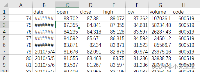
如图为茅台的股票数据
我们只用c列数据进行预测
用连续60天的开盘价预测第61天的开盘价

分析：

1.import
2.读取文件，划分train、test，归一化，生成整个数据集并乱序
3.model=tf.keras.Sequential(…)
4.model.compile(…)
5.断点续训，保存模型，model.fit(…)
6.model.summary()
7.参数提取（参数打印到txt文件）
8.acc/loss可视化
9.基于已有模型进行预测并把预测结构可视化
10.打印mse，rmse，mae等误差

代码：

import numpy as np
import tensorflow as tf
from tensorflow.keras.layers import Dropout, Dense, SimpleRNN
import matplotlib.pyplot as plt
import os
import pandas as pd
from sklearn.preprocessing import MinMaxScaler
from sklearn.metrics import mean_squared_error, mean_absolute_error
import math

maotai = pd.read_csv('./SH600519.csv')  # 读取股票文件

training_set = maotai.iloc[0:2426 - 300, 2:3].values  # 前(2426-300=2126)天的开盘价作为训练集,表格从0开始计数，2:3 是提取[2:3)列，前闭后开,故提取出C列开盘价
test_set = maotai.iloc[2426 - 300:, 2:3].values  # 后300天的开盘价作为测试集

# 归一化
sc = MinMaxScaler(feature_range=(0, 1))  # 定义归一化：归一化到(0，1)之间
training_set_scaled = sc.fit_transform(training_set)  # 求得训练集的最大值，最小值这些训练集固有的属性，并在训练集上进行归一化
test_set = sc.transform(test_set)  # 利用训练集的属性对测试集进行归一化

x_train = []
y_train = []

x_test = []
y_test = []

# 测试集：csv表格中前2426-300=2126天数据
# 利用for循环，遍历整个训练集，提取训练集中连续60天的开盘价作为输入特征x_train，第61天的数据作为标签，for循环共构建2426-300-60=2066组数据。
for i in range(60, len(training_set_scaled)):
    x_train.append(training_set_scaled[i - 60:i, 0])
    y_train.append(training_set_scaled[i, 0])
# 对训练集进行打乱
np.random.seed(7)
np.random.shuffle(x_train)
np.random.seed(7)
np.random.shuffle(y_train)
tf.random.set_seed(7)
# 将训练集由list格式变为array格式
x_train, y_train = np.array(x_train), np.array(y_train)

# 使x_train符合RNN输入要求：[送入样本数， 循环核时间展开步数， 每个时间步输入特征个数]。
# 此处整个数据集送入，送入样本数为x_train.shape[0]即2066组数据；输入60个开盘价，预测出第61天的开盘价，循环核时间展开步数为60; 每个时间步送入的特征是某一天的开盘价，只有1个数据，故每个时间步输入特征个数为1
x_train = np.reshape(x_train, (x_train.shape[0], 60, 1))
# 测试集：csv表格中后300天数据
# 利用for循环，遍历整个测试集，提取测试集中连续60天的开盘价作为输入特征x_train，第61天的数据作为标签，for循环共构建300-60=240组数据。
for i in range(60, len(test_set)):
    x_test.append(test_set[i - 60:i, 0])
    y_test.append(test_set[i, 0])
# 测试集变array并reshape为符合RNN输入要求：[送入样本数， 循环核时间展开步数， 每个时间步输入特征个数]
x_test, y_test = np.array(x_test), np.array(y_test)
x_test = np.reshape(x_test, (x_test.shape[0], 60, 1))

model = tf.keras.Sequential([
    SimpleRNN(80, return_sequences=True),
    Dropout(0.2),
    SimpleRNN(100),
    Dropout(0.2),
    Dense(1)
])

model.compile(optimizer=tf.keras.optimizers.Adam(0.001),
              loss='mean_squared_error')  # 损失函数用均方误差
# 该应用只观测loss数值，不观测准确率，所以删去metrics选项，一会在每个epoch迭代显示时只显示loss值

checkpoint_save_path = "./checkpoint/rnn_stock.ckpt"

if os.path.exists(checkpoint_save_path + '.index'):
    print('-------------load the model-----------------')
    model.load_weights(checkpoint_save_path)

cp_callback = tf.keras.callbacks.ModelCheckpoint(filepath=checkpoint_save_path,
                                                 save_weights_only=True,
                                                 save_best_only=True,
                                                 monitor='val_loss')

history = model.fit(x_train, y_train, batch_size=64, epochs=50, validation_data=(x_test, y_test), validation_freq=1,
                    callbacks=[cp_callback])

model.summary()

file = open('./weights.txt', 'w')  # 参数提取
for v in model.trainable_variables:
    file.write(str(v.name) + '\n')
    file.write(str(v.shape) + '\n')
    file.write(str(v.numpy()) + '\n')
file.close()

loss = history.history['loss']
val_loss = history.history['val_loss']

plt.plot(loss, label='Training Loss')
plt.plot(val_loss, label='Validation Loss')
plt.title('Training and Validation Loss')
plt.legend()
plt.show()

################## predict ######################
# 测试集输入模型进行预测
predicted_stock_price = model.predict(x_test)
# 对预测数据还原---从（0，1）反归一化到原始范围
predicted_stock_price = sc.inverse_transform(predicted_stock_price)
# 对真实数据还原---从（0，1）反归一化到原始范围
real_stock_price = sc.inverse_transform(test_set[60:])  # test_set[60:]也可换为y_test
# 画出真实数据和预测数据的对比曲线
plt.plot(real_stock_price, color='red', label='MaoTai Stock Price')
plt.plot(predicted_stock_price, color='blue', label='Predicted MaoTai Stock Price')
plt.title('MaoTai Stock Price Prediction')
plt.xlabel('Time')
plt.ylabel('MaoTai Stock Price')
plt.legend()
plt.show()

##########evaluate##############
# calculate MSE 均方误差 ---> E[(预测值-真实值)^2] (预测值减真实值求平方后求均值)
mse = mean_squared_error(predicted_stock_price, real_stock_price)
# calculate RMSE 均方根误差--->sqrt[MSE]    (对均方误差开方)
rmse = math.sqrt(mean_squared_error(predicted_stock_price, real_stock_price))
# calculate MAE 平均绝对误差----->E[|预测值-真实值|](预测值减真实值求绝对值后求均值）
mae = mean_absolute_error(predicted_stock_price, real_stock_price)
print('均方误差: %.6f' % mse)
print('均方根误差: %.6f' % rmse)
print('平均绝对误差: %.6f' % mae)

LSTM神经网络

RNN可以通过记忆体实现短期记忆进行连续数据的预测，但是当连续数据的序列变长时，会使展开时间步过长，在反向传播更新参数时，梯度要按时间步连续相乘，会导致梯度消失。
而LSTM通过门控制单元改善了RNN长期依赖的问题
LSTM（长短时记忆神经网络）引入了输入门（it）、遗忘门（ft）、输出门（ot）三个门限。引入表征长期记忆的细胞态Ct，等待存入长期记忆的候选态Ct~，以及此前RNN的记忆体ht
在这里插入图片描述
Wi,Wf,Wo,Wc,bi,bf,bo,bc是带训练参数，σ是sigmoid函数

Ct-1是以前的长期记忆，Ct~是现在准备记的东西（现在准备记的东西可能会受以前记忆的影响，所以里面包含有ht-1），现在的长期记忆Ct就是ft*Ct-1（表示以前的记忆忘了一部分）+it*Ct~（表示现在准备记的东西输入到脑子里面了，经过了输入门进入脑子），当我们回想自己的长期记忆时，不可能全部能回想起来，所以我们回想的时候需要加一个输出门，所以我们回想时的短期记忆是ht=ot*tanh(Ct)
当我们输出ht时，这个ht可以作为第二层循环网络的输入，即ht是第二层循环网络的xt

TF描述LSTM层：
tf.keras.layers.LSTM(记忆体个数，return_sequences=是否返回输出)
return_sequences=True 表示各时间步输出ht
return_sequences=False 表示仅最后实践输出ht（默认）
一般最后一层用False，中间层用True
如

model = tf.keras.Sequential([
    LSTM(80,return_sequences=True),
    Dropout(0.2),
    LSTM(100),
    Dropout(0.2),
    Dense(1)
])

LSTM预测股票价格：

只有以下部分和RNN不同，其余都是相同的：

from tensorflow.keras.layers import Dropout, Dense, LSTM

model = tf.keras.Sequential([
    LSTM(80, return_sequences=True),
    Dropout(0.2),
    LSTM(100),
    Dropout(0.2),
    Dense(1)
])

GRU神经网络

GRU神经网络是对LSTM的优化
在这里插入图片描述
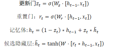
GRU使记忆体ht融合了长期记忆和短期记忆，ht包含了过去信息ht-1和现在信息ht_{，现在信息ht}是过去信息过重置门rt和当前输入xt共同决定的

TF描述GRU层
tf.keras.layers.GRU(记忆体个数，
return_sequences=是否返回输出)
return_sequences=True 表示各时间步输出ht
return_sequences=False 表示仅最后实践输出ht（默认）
一般最后一层用False，中间层用True
如

model = tf.keras.Sequential([
    GRU(80,return_sequences=True),
    Dropout(0.2),
    GRU(100),
    Dropout(0.2),
    Dense(1)
])

GRU预测股票价格：

只有以下部分和RNN不同，其余都是相同的：

from tensorflow.keras.layers import Dropout, Dense, GRU

model = tf.keras.Sequential([
    GRU(80, return_sequences=True),
    Dropout(0.2),
    GRU(100),
    Dropout(0.2),
    Dense(1)
])

牛+马=我

关注

0
点赞
踩
3

收藏

觉得还不错? 一键收藏
0
评论
循环神经网络（RNN）_6

用RNN实现连续数据的预测（以股票预测为例）目录：循环神经网络循环核循环核时间步展开循环计算层TF描述循环计算层循环计算过程实践：ABCDE字母预测One-hotEmbedding实践：股票预测RNNLSTMGRU
复制链接

扫一扫