Machine Learning-Ex8（吴恩达课后习题）Anomaly Detection and Recommender Systems

1. Anomaly detection

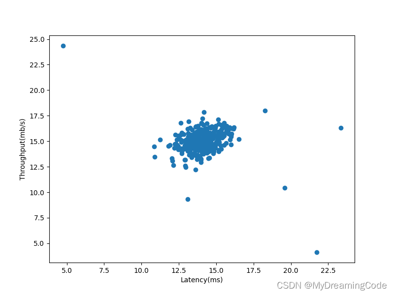
内容：使用高斯模型来检测数据集中异常的数据（概率低的），先在2维数据中进行实验。样本具有两个特征：a. 服务器响应的吞吐量（mb/s） b. 延迟（ms）。

数据可视化

main.py

from scipy.io import loadmat
import matplotlib.pyplot as plt

X = loadmat('ex8data1.mat')['X']
fig, ax = plt.subplots(figsize=(8, 6))
ax.scatter(X[:, 0], X[:, 1])
ax.set_xlabel('Latency(ms)')
ax.set_ylabel('Throughput(mb/s)')
plt.show()

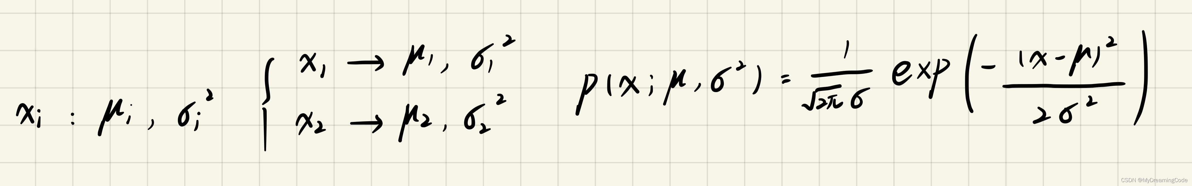
1.1 Gaussian distribution

内容：对每个特征  都拟合一个高斯分布。

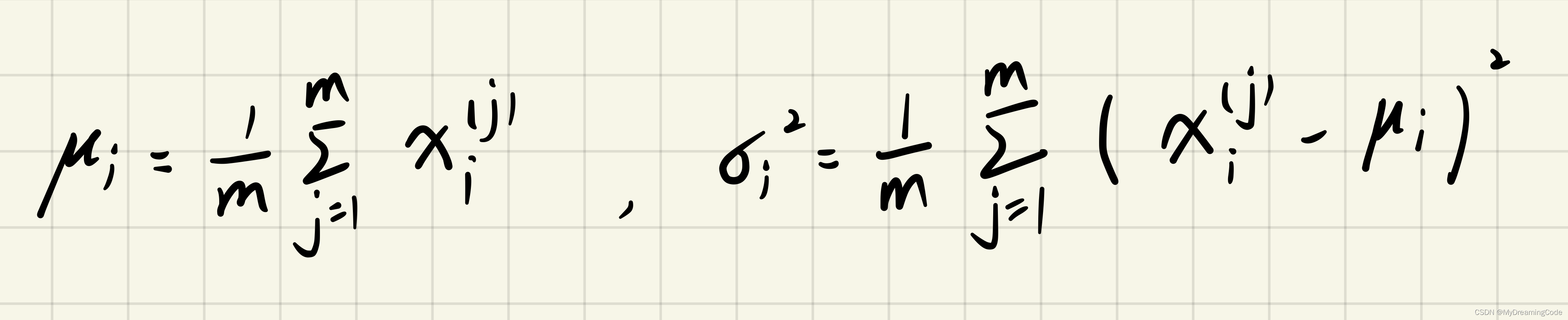
1.2 Estimating parameters for a Gaussian

内容：计算高斯分布函数的参数。输入一个X矩阵，得出一个包含n个特征的平均值mean和包含n个特征的sigma2。

estimateGaussian.py

def estimateGaussian(X):
    mean = X.mean(axis=0)
    sigma2 = X.var(axis=0)
    return mean, sigma2

main.py

from scipy.io import loadmat
from estimateGaussian import *  # 估算高斯分布的参数

X = loadmat('ex8data1.mat')['X']
mean, sigma2 = estimateGaussian(X)
print(mean, sigma2)

[14.11222578 14.99771051] [1.83263141 1.70974533]

数据可视化：

np.meshgrid为生成网络点坐标，如：

xplot = np.linspace(0, 25, 100)
yplot = np.linspace(0, 25, 100)
Xplot, Yplot = np.meshgrid(xplot, yplot)  # 生成网格点坐标
fig, ax = plt.subplots(figsize=(8, 6))
ax.scatter(Xplot, Yplot, s=5)
plt.show()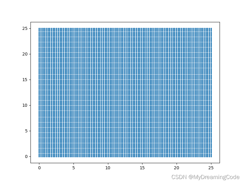

gaussianDistribution.py

import numpy as np

def gaussianDistribution(X, mean, sigma2):
    sigma2 = np.reshape(sigma2, (1, 2))
    mean = np.reshape(mean, (1, 2))
    p = (1 / (np.sqrt(2 * np.pi) * sigma2)) * (np.exp(-(X - mean) ** 2 / (2 * sigma2)))
    # prod为累乘
    return np.prod(p, axis=1)

main.py

from scipy.io import loadmat
import numpy as np
import matplotlib.pyplot as plt
from estimateGaussian import *  # 估算高斯分布的参数
from gaussianDistribution import *  # 计算高斯分布函数

X = loadmat('ex8data1.mat')['X']
fig, ax = plt.subplots(figsize=(8, 6))
ax.scatter(X[:, 0], X[:, 1])
mean, sigma2 = estimateGaussian(X)
gaussianDistribution(X, mean, sigma2)
xplot = np.linspace(0, 25, 100)
yplot = np.linspace(0, 25, 100)
Xplot, Yplot = np.meshgrid(xplot, yplot)  # 生成网格点坐标

# 1.concatenate用于拼接数组
# 2.reshape(-1,1) 转换成1列
X = np.concatenate((Xplot.reshape(-1, 1), Yplot.reshape(-1, 1)), axis=1)
p = gaussianDistribution(X, mean, sigma2).reshape(Xplot.shape)
# 3.绘制等高线
# contour(X,Y,Z,[levels]) levels:确定轮廓线的数量和位置
contour = plt.contour(Xplot, Yplot, p, [10 ** -11, 10 ** -7, 10 ** -5, 10 ** -3, 0.1])
ax.set_xlabel('Latency(ms)')
ax.set_ylabel('Throughput(mb/s)')
plt.show()

1.3 Selecting the threshold, ε

内容：根据交叉验证集，使用 F1-score 来选择合适的阈值ε。低概率的数据可能是异常的。

精确率（precision）召回率（recall）

                     

selectThreshold.py

import numpy as np

def selectThreshold(pval, yval):
    best_epsilon = 0
    best_f1 = 0
    f1 = 0
    step = (pval.max() - pval.min()) / 1000
    # 1.np.arange(start,end,step):step为步长
    # 2.np.logical_and(A,B) 返回A和B与逻辑后的布尔值
    for epsilon in np.arange(pval.min(), pval.max(), step):
        predicts = pval < epsilon  # anomaly
        # 虽然predicts(多一列)与yval列数不同，但是可以按照predicts的第一行与yval的第一行进行比较。
        tp = np.sum(np.logical_and(predicts == 1, yval == 1)).astype(float)
        fp = np.sum(np.logical_and(predicts == 1, yval == 0)).astype(float)
        fn = np.sum(np.logical_and(predicts == 0, yval == 1)).astype(float)
        prec = tp / (tp + fp) if tp + fp else 0
        rec = tp / (tp + fn) if tp + fn else 0
        f1 = (2 * prec * rec) / (prec + rec) if prec + rec else 0
        if f1 > best_f1:
            best_f1 = f1
            best_epsilon = epsilon
    return best_epsilon, best_f1

main.py 

from scipy.io import loadmat
from scipy import stats
import numpy as np
import matplotlib.pyplot as plt
from estimateGaussian import *  # 估算高斯分布的参数
from gaussianDistribution import *  # 计算高斯分布
from selectThreshold import *  # 选择阈值

raw_data = loadmat('ex8data1.mat')
X, Xval, yval = raw_data['X'], raw_data['Xval'], raw_data['yval']
mean, sigma2 = estimateGaussian(X)
# print(Xval.shape, yval.shape) (307, 2) (307, 1)
# 1.stats.norm(mean,sigma2).pdf:概率密度函数
p = np.zeros(X.shape)
p[:, 0] = stats.norm(mean[0], sigma2[0]).pdf(X[:, 0])
p[:, 1] = stats.norm(mean[1], sigma2[1]).pdf(X[:, 1])
# print(p.shape)  # (307, 2)
# 2.验证集在相同模型参数下计算概率
pval = np.zeros(Xval.shape)
pval[:, 0] = stats.norm(mean[0], sigma2[0]).pdf(Xval[:, 0])
pval[:, 1] = stats.norm(mean[1], sigma2[1]).pdf(Xval[:, 1])
# print(pval.shape)  # (307, 2)

epsilon, f1 = selectThreshold(pval, yval)
print(epsilon, f1)

0.009566706005956842 0.7142857142857143

可视化结果

main.py

from scipy.io import loadmat
from scipy import stats
import numpy as np
import matplotlib.pyplot as plt
from estimateGaussian import *  # 估算高斯分布的参数
from gaussianDistribution import *  # 计算高斯分布
from selectThreshold import *  # 选择阈值

raw_data = loadmat('ex8data1.mat')
X, Xval, yval = raw_data['X'], raw_data['Xval'], raw_data['yval']
mean, sigma2 = estimateGaussian(X)
# print(Xval.shape, yval.shape) (307, 2) (307, 1)
# 1.stats.norm(mean,sigma2).pdf:概率密度函数
p = np.zeros(X.shape)
p[:, 0] = stats.norm(mean[0], sigma2[0]).pdf(X[:, 0])
p[:, 1] = stats.norm(mean[1], sigma2[1]).pdf(X[:, 1])
# print(p.shape)  # (307, 2)
# 2.验证集在相同模型参数下计算概率
pval = np.zeros(Xval.shape)
pval[:, 0] = stats.norm(mean[0], sigma2[0]).pdf(Xval[:, 0])
pval[:, 1] = stats.norm(mean[1], sigma2[1]).pdf(Xval[:, 1])
# print(pval.shape)  # (307, 2)

epsilon, f1 = selectThreshold(pval, yval)
# np.where(A)返回符合条件元素的坐标
outliers = np.where(p < epsilon)[0]
# print(outliers)  # [300 301 301 303 303 304 306 306]

fig, ax = plt.subplots(figsize=(8, 6))
ax.scatter(X[:, 0], X[:, 1])
ax.scatter(X[outliers, 0], X[outliers, 1], c='r', marker='o')
ax.set_xlabel('Latency(ms)')
ax.set_ylabel('Throughput(mb/s)')
plt.show()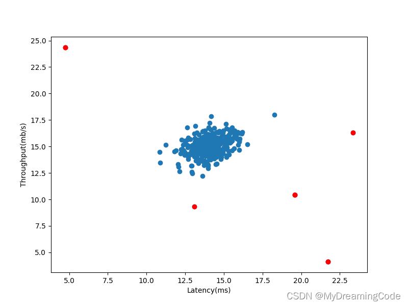

2. Recommender Systems

内容：该推荐系统将使用协同过滤算法在电影评级上进行应用。

2.1 Movie ratings dataset

内容：

n_movies：电影数量；n_users：用户数量

R(i,j)：值为1表示用户 j 对电影 i 评分过，0表示未评分

y(i,j)：评分（1-5），表示用户 j 对电影 i 的评分

矩阵：

X-电影的数据集（第 i 行表示由电影 i 组成的特征）

Theta-用户的数据集（第 j 行表示用户 j 对各类电影喜好程度的特征）

main.py 

from scipy.io import loadmat

data = loadmat('ex8_movies.mat')
Y, R = data['Y'], data['R']
# print(Y.shape, R.shape)  # (1682, 943) (1682, 943)
print(Y, R)

[[5 4 0 ... 5 0 0]
 [3 0 0 ... 0 0 5]
 [4 0 0 ... 0 0 0]
 ...
 [0 0 0 ... 0 0 0]
 [0 0 0 ... 0 0 0]
 [0 0 0 ... 0 0 0]] [[1 1 0 ... 1 0 0]
 [1 0 0 ... 0 0 1]
 [1 0 0 ... 0 0 0]
 ...
 [0 0 0 ... 0 0 0]
 [0 0 0 ... 0 0 0]
 [0 0 0 ... 0 0 0]]

评估电影的平均评级

main.py

from scipy.io import loadmat
import numpy as np

data = loadmat('ex8_movies.mat')
Y, R = data['Y'], data['R']
print(Y[1, np.where(R[1, :] == 1)].mean())
# 3.2061068702290076

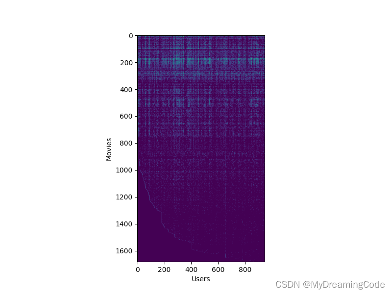
“可视化” 数据 

main.py

from scipy.io import loadmat
import matplotlib.pyplot as plt

data = loadmat('ex8_movies.mat')
Y, R = data['Y'], data['R']
fig, ax = plt.subplots(figsize=(8, 6))
ax.imshow(Y)
ax.set_xlabel('Users')
ax.set_ylabel('Movies')
plt.show()

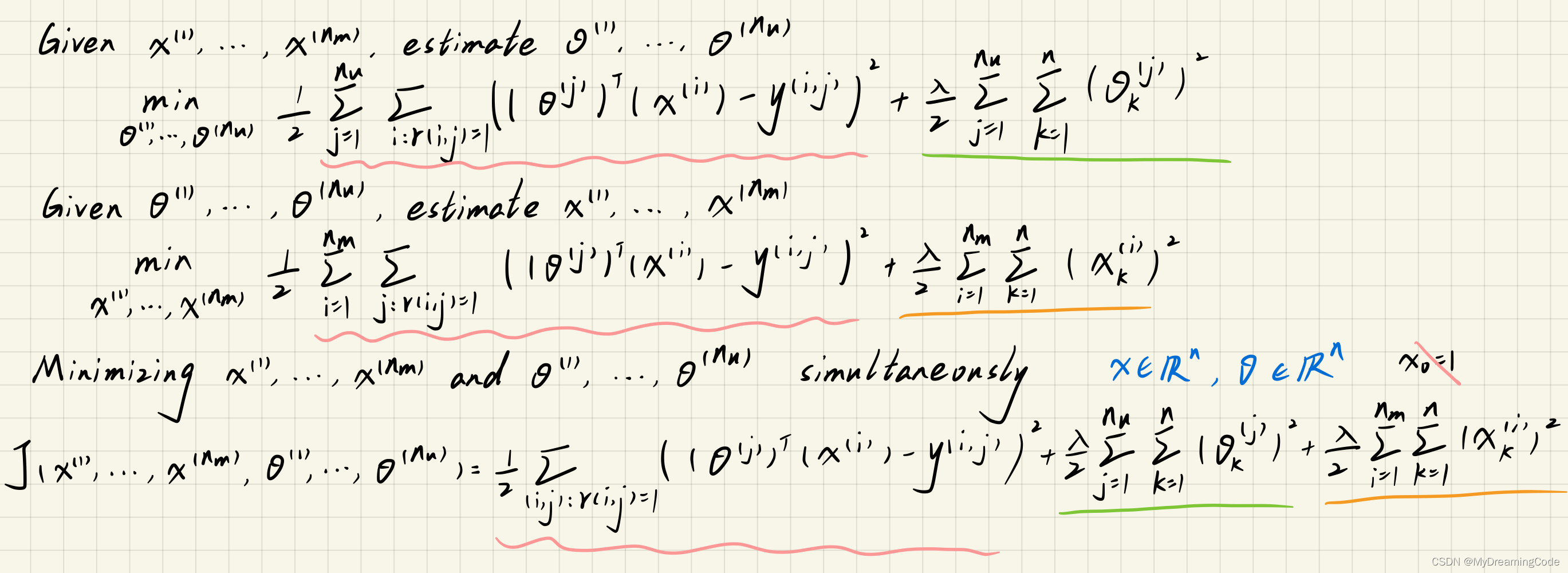
2.2 Collaborative filtering learning algorithm

内容：通过给定的一些用户评级电影的数据，并最小化代价函数，来学习参数X与Theta。

2.2.1 Collaborative filtering cost function

内容：

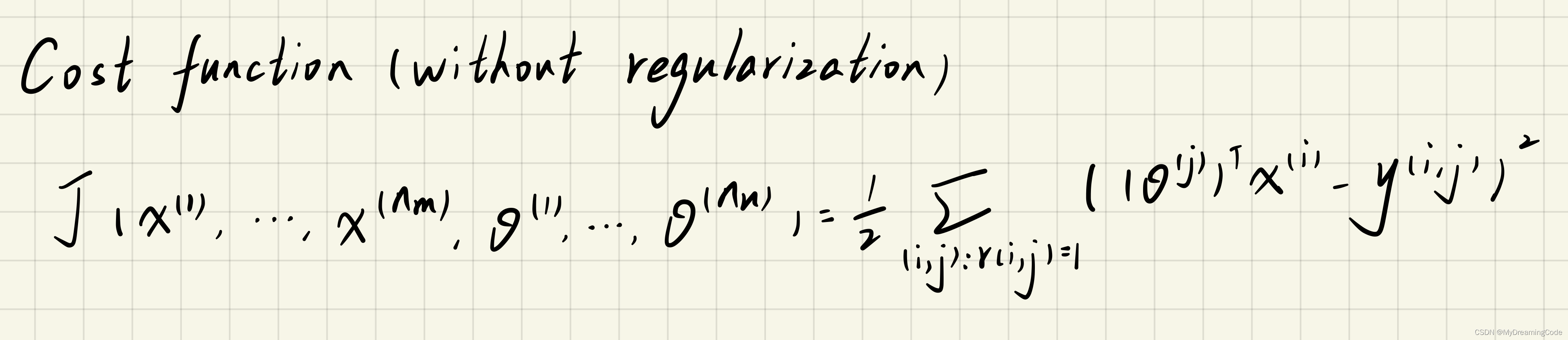
为了评估时间少一些，我们只取了少量的数据。（四位用户 五部电影 三个特征）

costFunction.py

import numpy as np

# 1.序列化
def serialize(X, theta):
    return np.concatenate((X.ravel(), theta.ravel()))

# 2.逆序列化
def deserialize(param, n_movies, n_users, n_features):
    return param[:n_movies * n_features].reshape(n_movies, n_features), param[n_movies * n_features:].reshape(n_users, n_features)

def costFunction(param, Y, R, n_features):
    n_movies, n_users = Y.shape
    X, theta = deserialize(param, n_movies, n_users, n_features)
    return np.sum(np.power(np.multiply(X @ theta.T - Y, R), 2)) / 2

main.py

from scipy.io import loadmat
from costFunction import *  # 代价函数

data = loadmat('ex8_movies.mat')
Y, R = data['Y'], data['R']
param_data = loadmat('ex8_movieParams.mat')
X, Theta = param_data['X'], param_data['Theta']
# 这里我们只取一小段数据
n_users = 4
n_movies = 5
n_features = 3
X_sub = X[:n_movies, :n_features]
Theta_sub = Theta[:n_users, :n_features]
Y_sub = Y[:n_movies, :n_users]
R_sub = R[:n_movies, :n_users]
param_sub = serialize(X_sub, Theta_sub)
print(costFunction(param_sub, Y_sub, R_sub, n_features))
param = serialize(X, Theta)
print(costFunction(param, Y, R, 10))

22.224603725685675
27918.64012454421

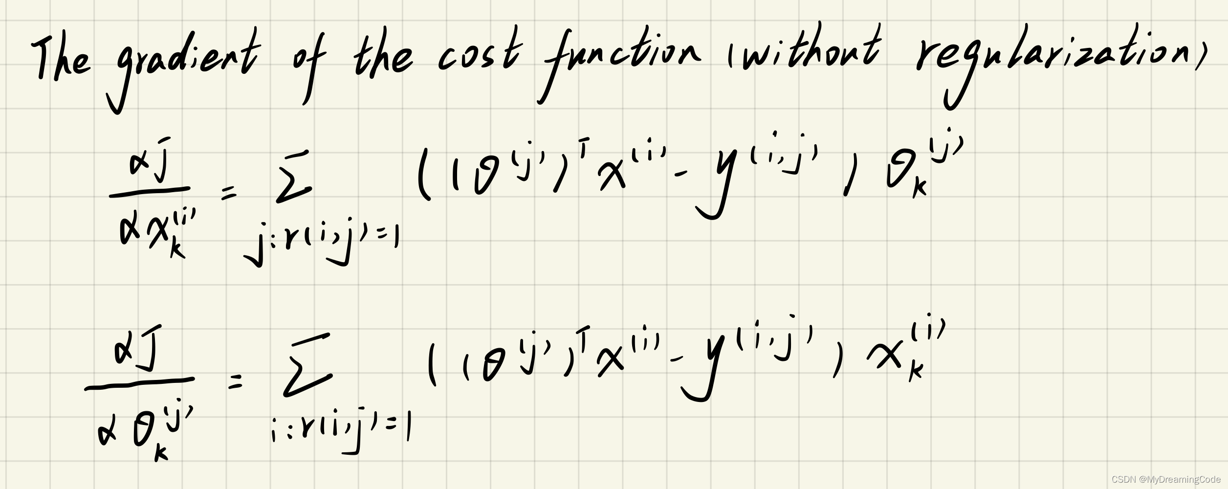
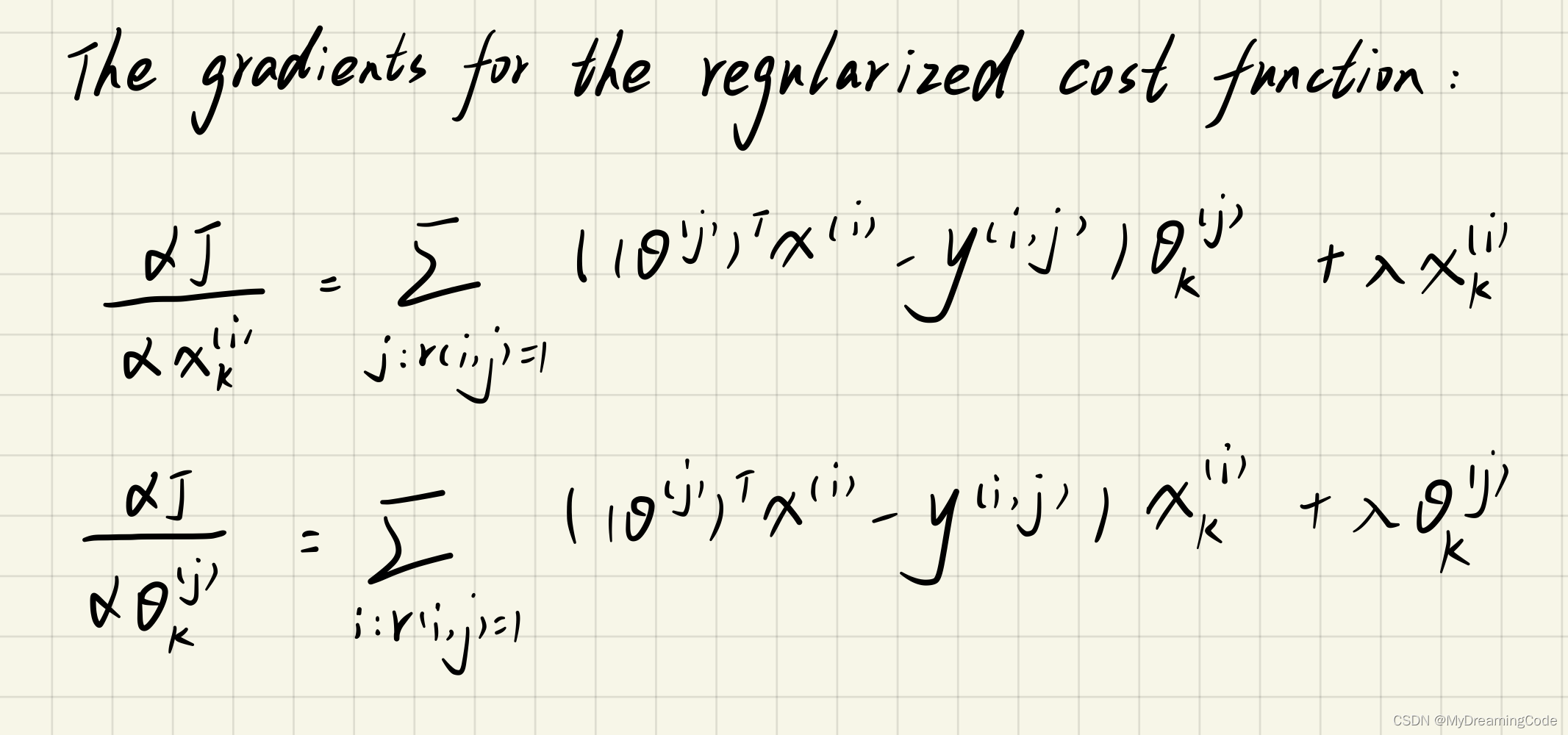
2.2.2 Collaborative filtering gradient

内容：计算梯度。

gradient.py

import numpy as np
from costFunction import *  # 序列化与逆序列化的方法

def gradient(param, Y, R, n_features):
    n_movies, n_users = Y.shape
    X, Theta = deserialize(param, n_movies, n_users, n_features)
    inner = np.multiply(X @ Theta.T - Y, R)
    X_grad = inner @ Theta
    Theta_grad = inner.T @ X
    return serialize(X_grad, Theta_grad)

main.py

from scipy.io import loadmat
from gradient import *  # 计算梯度

data = loadmat('ex8_movies.mat')
Y, R = data['Y'], data['R']
param_data = loadmat('ex8_movieParams.mat')
X, Theta = param_data['X'], param_data['Theta']
param = serialize(X, Theta)
n_movies, n_users = Y.shape
n_features = X.shape[1]
X_grad, Theta_grad = deserialize(gradient(param, Y, R, n_features), n_movies, n_users, n_features)
print(X_grad, Theta_grad)

[[-6.26184144  2.45936046 -6.87560329 ... -4.81611896  3.84341521
  -1.88786696]
 [-3.80931446  1.80494255 -2.63877955 ... -3.55580057  2.1709485
   2.65129032]
 [-3.13090116  2.54853961  0.23884578 ... -4.18778519  3.10538294
   5.47323609]
 ...
 [-1.04774171  0.99220776 -0.48920899 ... -0.75342146  0.32607323
  -0.89053637]
 [-0.7842118   0.76136861 -1.25614442 ... -1.05047808  1.63905435
  -0.14891962]
 [-0.38792295  1.06425941 -0.34347065 ... -2.04912884  1.37598855
   0.19551671]] [[-1.54728877  9.0812347  -0.6421836  ... -3.92035321  5.66418748
   1.16465605]
 [-2.58829914  2.52342335 -1.52402705 ... -5.46793491  5.82479897
   1.8849854 ]
 [ 2.14588899  2.00889578 -4.32190712 ... -6.83365682  1.78952063
   0.82886788]
 ...
 [-4.59816821  3.63958389 -2.52909095 ... -3.50886008  2.99859566
   0.64932177]
 [-4.39652679  0.55036362 -1.98451805 ... -6.74723702  3.8538775
   3.94901737]
 [-3.75193726  1.44393885 -5.6925333  ... -6.56073746  5.20459188
   2.65003952]]

2.2.3 Regularized cost function

内容：正则化代价函数

regularizedContent.py

import numpy as np
from costFunction import *  # 引入未正则化的代价函数

def regularizedCostFunction(param, Y, R, n_features, learningRate):
    reg = (learningRate / 2) * np.power(param, 2).sum()
    return costFunction(param, Y, R, n_features) + reg

main.py

from scipy.io import loadmat
from gradient import *  # 计算梯度
from regularizedContent import *  # 带正则化的代价函数和梯度计算

data = loadmat('ex8_movies.mat')
Y, R = data['Y'], data['R']
param_data = loadmat('ex8_movieParams.mat')
X, Theta = param_data['X'], param_data['Theta']
n_users = 4
n_movies = 5
n_features = 3
X_sub = X[:n_movies, :n_features]
Theta_sub = Theta[:n_users, :n_features]
Y_sub = Y[:n_movies, :n_users]
R_sub = R[:n_movies, :n_users]
param_sub = serialize(X_sub, Theta_sub)
learningRate = 1.5
print(regularizedCostFunction(param_sub, Y_sub, R_sub, n_features, learningRate))
param = serialize(X, Theta)
print(regularizedCostFunction(param, Y, R, 10, learningRate=1))

31.34405624427422
32520.682450229557

2.2.4 Regularized gradient

内容：正则化梯度。

regularizedContent.py

import numpy as np
from costFunction import *  # 引入未正则化的代价函数
from gradient import *  # 引入未正则化的梯度计算

def regularizedCostFunction(param, Y, R, n_features, learningRate):
    reg = (learningRate / 2) * np.power(param, 2).sum()
    return costFunction(param, Y, R, n_features) + reg

def regularizedGradient(param, Y, R, n_features, learningRate):
    grad = gradient(param, Y, R, n_features)
    reg = learningRate * param
    return grad + reg

main.py

from scipy.io import loadmat
from gradient import *  # 计算梯度
from regularizedContent import *  # 带正则化的代价函数和梯度计算

data = loadmat('ex8_movies.mat')
Y, R = data['Y'], data['R']
param_data = loadmat('ex8_movieParams.mat')
X, Theta = param_data['X'], param_data['Theta']
n_movies, n_users = Y.shape
param = serialize(X, Theta)
learningRate = 1
X_grad, Theta_grad = deserialize(regularizedGradient(param, Y, R, 10, learningRate), n_movies, n_users, 10)
print(X_grad, Theta_grad)

[[-5.21315594  2.0591285  -5.68148384 ... -3.95439796  3.14612528
  -1.59912133]
 [-3.02846323  1.41931663 -2.11758176 ... -2.85177984  1.68511329
   2.08666626]
 [-2.4893923   2.00068576  0.1550494  ... -3.34923876  2.41055086
   4.33843977]
 ...
 [-0.82821934  0.7917289  -0.39662935 ... -0.60746963  0.28294163
  -0.71223186]
 [-0.62377152  0.60121466 -1.02043496 ... -0.84313998  1.30670669
  -0.10603832]
 [-0.31115177  0.86705203 -0.2616062  ... -1.64900127  1.08850949
   0.16318173]] [[-1.26184516  7.39696961 -0.37924484 ... -3.15312086  4.55958584
   0.91278897]
 [-2.08328593  2.06877489 -1.20656461 ... -4.37487155  4.62450461
   1.49336864]
 [ 1.71397243  1.53009129 -3.47519602 ... -5.47031706  1.46428521
   0.63418576]
 ...
 [-3.53947561  2.83086629 -1.95973324 ... -2.70464586  2.25512788
   0.52946291]
 [-3.50593747  0.42141628 -1.62891338 ... -5.37296895  3.1012226
   3.13766426]
 [-2.92779591  1.05501291 -4.62312829 ... -5.27650042  4.22109195
   2.11819114]]

2.3 Learning movie recommendations

内容：创建自己的电影评分，以生成个性化推荐。有一个提供连接电影索引到其标题的文件。

main.py

import numpy as np

# open打开一个文件
f = open('movie_ids.txt', encoding='gbk', errors='ignore')
movie_list = []
for line in f:
    tokens = line.strip().split(' ')
    movie_list.append(' '.join(tokens[1:]))  # 将电影名存入列表中
movie_list = np.array(movie_list)
print(movie_list[0])

Toy Story (1995)

2.3.1 Recommendations

内容：将自己的评级数据添加到原始数据中。训练数据，得到参数，推荐出用户可能喜欢的电影。

首先演示一下Python插入数据（非0即1，0则0）

test.py

import numpy as np

arr = np.array([
    [1, 1, 1],
    [1, 1, 0],
    [1, 1, 0]
]).reshape(3, 3)
rate = np.array([2, 3, 0]).reshape(3, 1)
arr = np.append(rate != 0, arr, axis=1)
print(arr)

[[1 1 1 1]
 [1 1 1 0]
 [0 1 1 0]] 

对评级进行归一化处理，并训练数据。

main.py

import numpy as np
from scipy.io import loadmat
from scipy.optimize import minimize
from costFunction import *
from regularizedContent import *

# open打开一个文件
f = open('movie_ids.txt', encoding='gbk', errors='ignore')
movie_list = []
for line in f:
    tokens = line.strip().split(' ')
    movie_list.append(' '.join(tokens[1:]))  # 将电影名存入列表中
movie_list = np.array(movie_list)

ratings = np.zeros((1682, 1))  # 给定一些电影的评分
ratings[0] = 4
ratings[6] = 3
ratings[11] = 5
ratings[65] = 3
ratings[68] = 5
ratings[97] = 2
ratings[182] = 4
ratings[225] = 5
ratings[354] = 5
# print(ratings.shape)  # (1682, 1)

# 1.我们现在成为user0
raw_data = loadmat('ex8_movies')
Y, R = raw_data['Y'], raw_data['R']
Y = np.append(ratings, Y, axis=1)
# print(Y.shape)
R = np.append(ratings != 0, R, axis=1)
# print(R.shape)  # (1682, 944)

n_movies, n_users = Y.shape
n_features = 10
learningRate = 10
# 2.初始化X,Theta参数
# np.random.random((a,b))-生成a行b列的浮点数(0-1随机)
X = np.random.random((n_movies, n_features))
Theta = np.random.random((n_users, n_features))
param = serialize(X, Theta)
# print(X.shape, Theta.shape, param.shape)  # (1682, 10) (944, 10) (26260,)

# 3.进行归一化
Y_mean = (Y.sum(axis=1) / R.sum(axis=1)).reshape(-1, 1)
# print(Y_mean.shape)  # (1682, 1)
Y_norm = np.multiply(Y - Y_mean, R)
# print(Y_norm.shape)  # (1682, 944)

# 4.训练数据
fmin = minimize(fun=regularizedCostFunction, x0=param, args=(Y_norm, R, n_features, learningRate), method='TNC',
                jac=regularizedGradient)
X_trained, Theta_trained = deserialize(fmin.x, n_movies, n_users, n_features)
# print(X_trained.shape, theta_trained.shape)  # (1682, 10) (944, 10)

# 5.得到训练出的数据后，给出所推荐的电影
predictions = X_trained @ Theta_trained.T
# print(predictions.shape)  # (1682, 944)
Y_mean = (Y.sum(axis=1) / R.sum(axis=1))
my_preds = predictions[:, 0] + Y_mean
# print(my_preds.shape)  # (1682,)
# argsort返回数组值从小到大的索引值
idx = np.argsort(my_preds)[::-1]  # 降序排列
for m in movie_list[idx][:5]:
    print(m)  # 取前五部高分的

Santa with Muscles (1996)
Great Day in Harlem, A (1994)
Entertaining Angels: The Dorothy Day Story (1996)
They Made Me a Criminal (1939)
Saint of Fort Washington, The (1993)