深度学习训练营之鸟类识别

原文链接

• 🍨 本文为🔗365天深度学习训练营 中的学习记录博客
• 🍦 参考文章：365天深度学习训练营-第P8周：实现鸟类识别
• 🍖 原作者：K同学啊|接辅导、项目定制

环境介绍

• 语言环境：Python3.9.13
• 编译器：jupyter notebook
• 深度学习环境：TensorFlow2

前置工作

设置GPU

使用gpu可以加快运行速度

#设置gpu
import tensorflow as tf

gpus = tf.config.list_physical_devices("GPU")

if gpus:
    tf.config.experimental.set_memory_growth(gpus[0], True)  #设置GPU显存用量按需使用
    tf.config.set_visible_devices([gpus[0]],"GPU")

导入数据并进行查找

# 导入数据
import matplotlib.pyplot as plt
# 支持中文
plt.rcParams['font.sans-serif'] = ['SimHei']  # 用来正常显示中文标签
plt.rcParams['axes.unicode_minus'] = False  # 用来正常显示负号

import os,PIL

# 设置随机种子尽可能使结果可以重现
import numpy as np
np.random.seed(1)

# 设置随机种子尽可能使结果可以重现
import tensorflow as tf
tf.random.set_seed(1)

from tensorflow import keras
from tensorflow.keras import layers,models

import pathlib

查看数据

data_dir = "D:/BaiduNetdiskDownload/第8天-没有加密版本/第8天/bird_photos"

data_dir = pathlib.Path(data_dir)
#3. 查看数据
image_count = len(list(data_dir.glob('*/*')))

print("图片总数为：",image_count)

我们可以知道一共有565张照片

数据处理

文件夹	数量
Bananaquit	166 张
Black Throated Bushtiti	111 张
Black skimmer	122 张
Cockatoo	166张

对数据进行加载操作
使用image_dataset_from_directory方法将磁盘中的数据加载到tf.data.Dataset中

batch_size = 8
img_height = 224
img_width = 224

"""
关于image_dataset_from_directory()的详细介绍可以参考文章：https://mtyjkh.blog.csdn.net/article/details/117018789
"""
train_ds = tf.keras.preprocessing.image_dataset_from_directory(
    data_dir,
    validation_split=0.2,
    subset="training",
    seed=123,
    image_size=(img_height, img_width),
    batch_size=batch_size)
#使用当中的452张进行训练

使用当中的452张进行训练

"""
关于image_dataset_from_directory()的详细介绍可以参考文章：https://mtyjkh.blog.csdn.net/article/details/117018789
"""
val_ds = tf.keras.preprocessing.image_dataset_from_directory(
    data_dir,
    validation_split=0.2,
    subset="validation",
    seed=123,
    image_size=(img_height, img_width),
    batch_size=batch_size)

使用113张进行预测操作

# 使用class_name输出数据集的标签
class_names = train_ds.class_names
print(class_names)

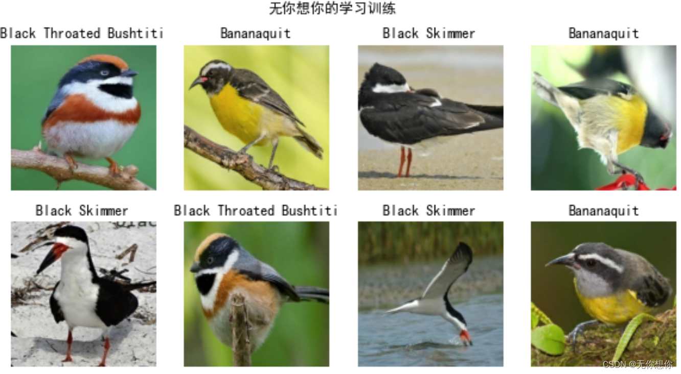
可视化数据

plt.figure(figsize=(10, 5))  # 图形的宽为10高为5
plt.suptitle("无你想你的学习训练")

for images, labels in train_ds.take(1):
    for i in range(8):
        
        ax = plt.subplot(2, 4, i + 1)  

        plt.imshow(images[i].numpy().astype("uint8"))
        plt.title(class_names[labels[i]])
        
        plt.axis("off")

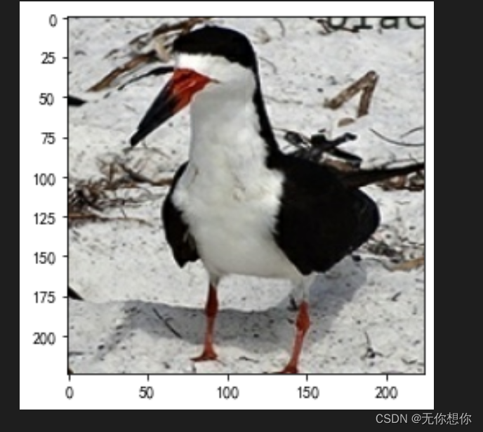
plt.imshow(images[4].numpy().astype("uint8"))

再次对数据进行检查

for image_batch, labels_batch in train_ds:
    print(image_batch.shape)
    print(labels_batch.shape)
    break

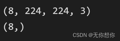
• Image_batch是形状的张量（8, 224, 224, 3)。这是一批形状240x240x3的8张图片（最后一维指的是彩色通道RGB）。
• Label_batch是形状（8，）的张量，这些标签对应8张图片

配置数据集

• shuffle() ：打乱数据，关于此函数的详细介绍可以参考：https://zhuanlan.zhihu.com/p/42417456
• prefetch() ：预取数据，加速运行，其详细介绍可以参考我前两篇文章，里面都有讲解。
• cache() ：将数据集缓存到内存当中，加速运行

AUTOTUNE = tf.data.AUTOTUNE

train_ds = train_ds.cache().shuffle(1000).prefetch(buffer_size=AUTOTUNE)
val_ds = val_ds.cache().prefetch(buffer_size=AUTOTUNE)

残差网络的介绍

残差网络是为了解决神经网络隐藏层过多时，而引起的网络退化问题。退化（degradation）问题是指：当网络隐藏层变多时，网络的准确度达到饱和然后急剧退化，而且这个退化不是由于过拟合引起的。

构建残差网络

from keras import layers

from keras.layers import Input,Activation,BatchNormalization,Flatten
from keras.layers import Dense,Conv2D,MaxPooling2D,ZeroPadding2D,AveragePooling2D
from keras.models import Model

def identity_block(input_tensor, kernel_size, filters, stage, block):

    filters1, filters2, filters3 = filters

    name_base = str(stage) + block + '_identity_block_'

    x = Conv2D(filters1, (1, 1), name=name_base + 'conv1')(input_tensor)
    x = BatchNormalization(name=name_base + 'bn1')(x)
    x = Activation('relu', name=name_base + 'relu1')(x)

    x = Conv2D(filters2, kernel_size,padding='same', name=name_base + 'conv2')(x)
    x = BatchNormalization(name=name_base + 'bn2')(x)
    x = Activation('relu', name=name_base + 'relu2')(x)

    x = Conv2D(filters3, (1, 1), name=name_base + 'conv3')(x)
    x = BatchNormalization(name=name_base + 'bn3')(x)

    x = layers.add([x, input_tensor] ,name=name_base + 'add')
    x = Activation('relu', name=name_base + 'relu4')(x)
    return x


def conv_block(input_tensor, kernel_size, filters, stage, block, strides=(2, 2)):

    filters1, filters2, filters3 = filters

    res_name_base = str(stage) + block + '_conv_block_res_'
    name_base = str(stage) + block + '_conv_block_'

    x = Conv2D(filters1, (1, 1), strides=strides, name=name_base + 'conv1')(input_tensor)
    x = BatchNormalization(name=name_base + 'bn1')(x)
    x = Activation('relu', name=name_base + 'relu1')(x)

    x = Conv2D(filters2, kernel_size, padding='same', name=name_base + 'conv2')(x)
    x = BatchNormalization(name=name_base + 'bn2')(x)
    x = Activation('relu', name=name_base + 'relu2')(x)

    x = Conv2D(filters3, (1, 1), name=name_base + 'conv3')(x)
    x = BatchNormalization(name=name_base + 'bn3')(x)

    shortcut = Conv2D(filters3, (1, 1), strides=strides, name=res_name_base + 'conv')(input_tensor)
    shortcut = BatchNormalization(name=res_name_base + 'bn')(shortcut)

    x = layers.add([x, shortcut], name=name_base+'add')
    x = Activation('relu', name=name_base+'relu4')(x)
    return x

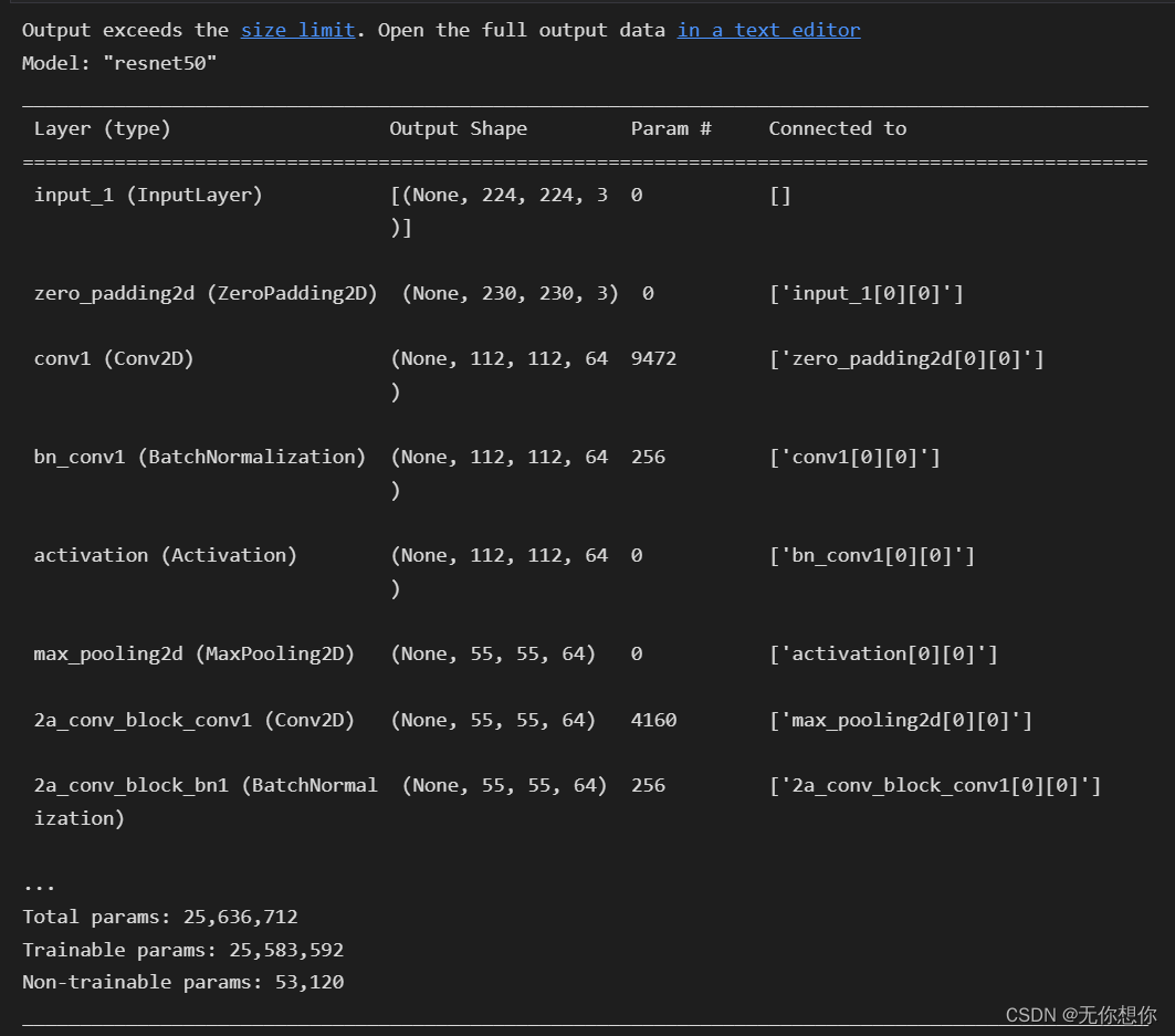
def ResNet50(input_shape=[224,224,3],classes=1000):

    img_input = Input(shape=input_shape)
    x = ZeroPadding2D((3, 3))(img_input)

    x = Conv2D(64, (7, 7), strides=(2, 2), name='conv1')(x)
    x = BatchNormalization(name='bn_conv1')(x)
    x = Activation('relu')(x)
    x = MaxPooling2D((3, 3), strides=(2, 2))(x)

    x =     conv_block(x, 3, [64, 64, 256], stage=2, block='a', strides=(1, 1))
    x = identity_block(x, 3, [64, 64, 256], stage=2, block='b')
    x = identity_block(x, 3, [64, 64, 256], stage=2, block='c')

    x =     conv_block(x, 3, [128, 128, 512], stage=3, block='a')
    x = identity_block(x, 3, [128, 128, 512], stage=3, block='b')
    x = identity_block(x, 3, [128, 128, 512], stage=3, block='c')
    x = identity_block(x, 3, [128, 128, 512], stage=3, block='d')

    x =     conv_block(x, 3, [256, 256, 1024], stage=4, block='a')
    x = identity_block(x, 3, [256, 256, 1024], stage=4, block='b')
    x = identity_block(x, 3, [256, 256, 1024], stage=4, block='c')
    x = identity_block(x, 3, [256, 256, 1024], stage=4, block='d')
    x = identity_block(x, 3, [256, 256, 1024], stage=4, block='e')
    x = identity_block(x, 3, [256, 256, 1024], stage=4, block='f')

    x =     conv_block(x, 3, [512, 512, 2048], stage=5, block='a')
    x = identity_block(x, 3, [512, 512, 2048], stage=5, block='b')
    x = identity_block(x, 3, [512, 512, 2048], stage=5, block='c')

    x = AveragePooling2D((7, 7), name='avg_pool')(x)

    x = Flatten()(x)
    x = Dense(classes, activation='softmax', name='fc1000')(x)

    model = Model(img_input, x, name='resnet50')
    
    # 加载预训练模型
    model.load_weights("resnet50_weights_tf_dim_ordering_tf_kernels.h5")

    return model

model = ResNet50()
model.summary()

模型训练

开始编译

• 损失函数（loss）：用于衡量模型在训练期间的准确率。
• 优化器（optimizer）：决定模型如何根据其看到的数据和自身的损失函数进行更新。
• 指标（metrics）：用于监控训练和测试步骤。以下示例使用了准确率，即被正确分类的图像的比率

# 设置优化器，我这里改变了学习率。
opt = tf.keras.optimizers.Adam(learning_rate=1e-7)

model.compile(optimizer="adam",
              loss='sparse_categorical_crossentropy',
              metrics=['accuracy'])

开始训练

epochs = 10

history = model.fit(
    train_ds,
    validation_data=val_ds,
    epochs=epochs
)

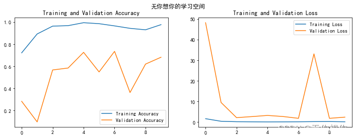
结果可视化

训练样本和测试样本

acc = history.history['accuracy']
val_acc = history.history['val_accuracy']

loss = history.history['loss']
val_loss = history.history['val_loss']

epochs_range = range(epochs)

plt.figure(figsize=(12, 4))
plt.subplot(1, 2, 1)
plt.suptitle("无你想你的学习空间")

plt.plot(epochs_range, acc, label='Training Accuracy')
plt.plot(epochs_range, val_acc, label='Validation Accuracy')
plt.legend(loc='lower right')
plt.title('Training and Validation Accuracy')

plt.subplot(1, 2, 2)
plt.plot(epochs_range, loss, label='Training Loss')
plt.plot(epochs_range, val_loss, label='Validation Loss')
plt.legend(loc='upper right')
plt.title('Training and Validation Loss')
plt.show()

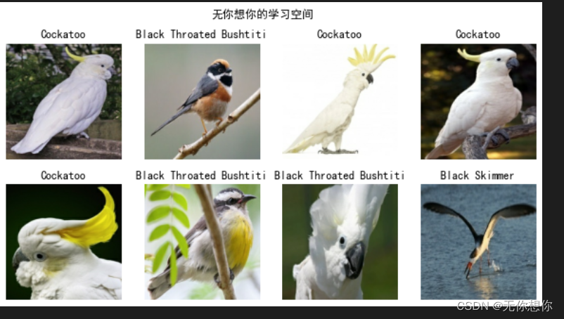
预测

# 保存模型
model.save('model/my_model.h5')

# 加载模型
new_model = keras.models.load_model('model/my_model.h5')

# 采用加载的模型（new_model）来看预测结果

plt.figure(figsize=(10, 5))  # 图形的宽为10高为5
plt.suptitle("无你想你的学习空间")

for images, labels in val_ds.take(1):
    for i in range(8):
        ax = plt.subplot(2, 4, i + 1)  
        
        # 显示图片
        plt.imshow(images[i].numpy().astype("uint8"))
        
        # 需要给图片增加一个维度
        img_array = tf.expand_dims(images[i], 0) 
        
        # 使用模型预测图片中的人物
        predictions = new_model.predict(img_array)
        plt.title(class_names[np.argmax(predictions)])

        plt.axis("off")