咖啡豆识别

最新推荐文章于 2024-05-10 19:20:28 发布

我也不太懂

最新推荐文章于 2024-05-10 19:20:28 发布

阅读量130

点赞数

文章标签： tensorflow 深度学习人工智能

本文链接：https://blog.csdn.net/qq_66033623/article/details/130741396

版权

本文为🔗365天深度学习训练营中的学习记录博客
原作者：K同学啊|接辅导、项目定制

我的环境：

1.语言：python3.7

2.编译器：pycharm

3.深度学习环境：TensorFlow2.5

一.前期工作

1.设置GPU

若是使用的是cpu可忽略

import tensorflow as tf
gpus = tf.config.list_physical_devices("GPU")

if gpus:
    gpu0 = gpus[0]
    tf.config.experimental.set_memory_growth(gpu0, True)
    tf.config.set_visible_devices([gpu0],"GPU")

使用cpu训练

import os
os.environ["CUDA_VISIBLE_DEVICES"] = "-1"

2.导入数据集

from tensorflow import keras
from tensorflow.keras import layers, models
import os, PIL, pathlib
import matplotlib.pyplot as plt
import tensorflow as tf
import numpy as np
 
data_dir = "E:/TF环境/49-data/"
data_dir = pathlib.Path(data_dir)

与前几次的学习任务一样，本次也是使用了pathlib模块，将data_dir中存储的路径传递给pathlib.Path类型的对象。方便我们对文件路径进行操作。

image_count = len(list(data_dir.glob('*/*.png')))
 
print("图片总数为：",image_count)

展示数据

打开Light下的第二张图片


roses = list(data_dir.glob('sunrise\*.jpg'))
PIL.Image.open(str(roses[1]))
ff = PIL.Image.open(str(roses[1]))
ff.show()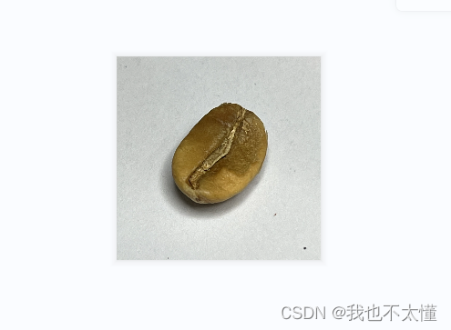

二、数据预处理

1、加载数据

图片格式设置

batch_size = 32
img_height = 224
img_width = 224

训练集、测试集和验证集的关系：
(1) 训练集相当于课后的练习题，用于日常的知识巩固。

(2) 验证集相当于周考，用来纠正和强化学到的知识。

(3) 测试集相当于期末考试，用来最终评估学习效果。

划分训练集：
使用image_dataset_from_directory方法将磁盘中的数据加载到tf.data.Dataset中。（可参考）

batch_size: 数据批次的大小。默认值：32
image_size: 从磁盘读取数据后将其重新调整大小。默认：（256，256）。由于管道处理的图像批次必须具有相同的大小，因此该参数必须提供。
seed: 用于shuffle和转换的可选随机种子。
tf.keras.preprocessing.image_dataset_from_directory() 简介

train_ds = tf.keras.preprocessing.image_dataset_from_directory(
    data_dir,
    validation_split=0.2,
    subset="training",
    label_mode = "categorical",
    seed = 123,
    image_size = (img_height, img_width),
    batch_size = batch_size
)

划分验证集：

验证集虽然没有直接参与模型的训练过程，但是为我们增加了一个人工调试的环节。我们可以根据每一轮的训练在测试集上的表现来决定是否需要训练进行early stop，还可以根据这个过程来调整模型的超参。

val_ds = tf.keras.preprocessing.image_dataset_from_directory(
    data_dir,
    validation_split=0.2,
    subset="validation",
    label_mode = "categorical",
    seed = 123,
    image_size = (img_height, img_width),
    batch_size = batch_size
)

查看标签

class_names = train_ds.class_names
print(class_names)

train_ds.class_names 是一个属性，它是通过数据集对象 train_ds 中的类别信息自动生成的一个包含类别名称的列表。

2、可视化数据

plt.figure(figsize = (20, 10))# 创建一个画布，画布大小为宽20、高10(单位为英寸inch)
for images, labels in train_ds.take(1):
  for i in range(10):
    ax = plt.subplot(2, 5, i + 1)
    plt.imshow(images[i].numpy().astype("uint8"))
    plt.title(class_names[np.argmax(labels[i])])
    plt.axis("off")
plt.show()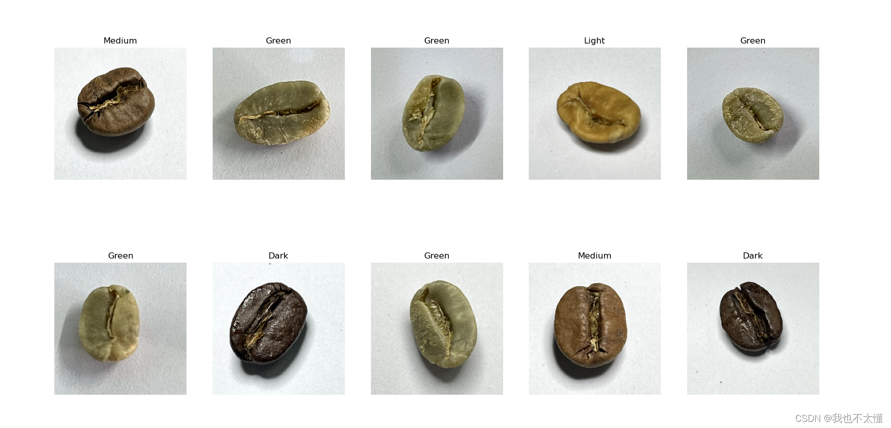

3、再次检查数据

for image_batch, labels_batch in train_ds:
  print(image_batch.shape)
  print(labels_batch.shape)
  break

image_batch是形状的张量（32，224，224，3）.这是一批形状224x224x3的32张图片（最后一维是指彩色通道RGB）。

label_batch是形状（32，）的张量，这些标签对应32张图片

4、配置数据集

AUTOTUNE = tf.data.AUTOTUNE
train_ds = train_ds.cache().shuffle(1000).prefetch(buffer_size=AUTOTUNE)
val_ds = val_ds.cache().prefetch(buffer_size=AUTOTUNE)


normalization_layer = layers.experimental.preprocessing.Rescaling(1./255)
train_ds = train_ds.map(lambda x,y:(normalization_layer(x),y))
val_ds = val_ds.map(lambda x,y:normalization_layer(x),y)
 
iamge_batch ,labels_batch = next(iter(train_ds))
first_image = image_batch[0]
print(np.min(first_image),np.max(first_image))

AUTOTUNE 是 TensorFlow 的一个常量。它表示 TensorFlow 数据处理流程中可以自动选择最优化参数（例如 GPU 处理数量等）的范围，在不同的硬件配置下可能会有不同的取值。

train_ds.cache() 和 val_ds.cache() 函数是 Tensorflow 的数据转换函数，它们的作用是将数据集中的元素缓存到内存或者磁盘中，以便后续访问时能够更快地读取数据。使用缓存可以避免由于磁盘 I/O 等因素导致数据读取速度变慢的问题，从而加速训练或评估过程。

train_ds.shuffle(1000) 函数是 Tensorflow 的数据转换函数，它的作用是将输入数据集中的元素随机打乱顺序。
这样做的目的是防止模型过拟合，并促进模型对不同数据的学习能力。其中，1000 表示用于对数据集进行重排的元素数量，其具体取值可以根据数据集大小进行调整。

shuffle（）：打乱数据。

prefetch（）：预取数据，加速运算。

cache（）：将数据集缓存到内存中，加速运行。

三、构建VGG-16网络

1、官方模型

#model = tk.keras.applications.VGG16(weights = 'imagenet')
#model.summary()

2、自建模型

from tensorflow.keras import layers,models,Input
from tensorflow.keras.models import Model
from tensorflow.keras.layers import Conv2D,MaxPooling2D,Dense,Flatten,Dropout
def VGG16(nb_classes, input_shape):
    input_tensor = Input(shape=input_shape)
    x = Conv2D(64,(3,3),activation='relu',padding='same',name='block1_conv1')(input_tensor)
    x = Conv2D(64,(3,3),activation='relu',padding='same',name='block1_conv2')(x)
    x = MaxPooling2D((2,2),strides=(2,2),name='block1_pool')(x)
    x = Conv2D(128,(3,3),activation='relu',padding='same',name='block2_conv1')(x)
    x = Conv2D(128,(3,3),activation='relu',padding='same',name='block2_conv2')(x)
    x = MaxPooling2D((2, 2), strides=(2, 2), name='block2_pool')(x)
    x = Conv2D(256, (3, 3), activation='relu', padding='same', name='block3_conv1')(x)
    x = Conv2D(256, (3, 3), activation='relu', padding='same', name='block3_conv2')(x)
    x = Conv2D(256, (3, 3), activation='relu', padding='same', name='block3_conv3')(x)
    x = MaxPooling2D((2, 2), strides=(2, 2), name='block3_pool')(x)
    x = Conv2D(512, (3, 3), activation='relu', padding='same', name='block4_conv1')(x)
    x = Conv2D(512, (3, 3), activation='relu', padding='same', name='block4_conv2')(x)
    x = Conv2D(512, (3, 3), activation='relu', padding='same', name='block4_conv3')(x)
    x = MaxPooling2D((2, 2), strides=(2, 2), name='block4_pool')(x)
    x = Conv2D(512, (3, 3), activation='relu', padding='same', name='block5_conv1')(x)
    x = Conv2D(512, (3, 3), activation='relu', padding='same', name='block5_conv2')(x)
    x = Conv2D(512, (3, 3), activation='relu', padding='same', name='block5_conv3')(x)
    x = MaxPooling2D((2, 2), strides=(2, 2), name='block5_pool')(x)
    x = Flatten()(x)
    x = Dense(4096,activation='relu',name='fc1')(x)
    x = Dense(4096, activation='relu', name='fc2')(x)
    output_tensor = Dense(nb_classes,activation='softmax',name='predictions')(x)
    model = Model(input_tensor,output_tensor)
    return model

model = VGG16(len(class_names),(img_width,img_height,3))
model.summary()

VGG优缺点分析：

VGG优点

VGG的结构很简洁，整个网络都使用了同样大小的卷积核尺寸（3x3）和最大池化尺寸（2x2）.

VGG缺点

1、训练时间过长。调参难度大。

2、需要的存储容量大，不利于部署。

Model: "model"
_________________________________________________________________
Layer (type)                 Output Shape              Param #   
=================================================================
input_1 (InputLayer)         [(None, 224, 224, 3)]     0         
_________________________________________________________________
block1_conv1 (Conv2D)        (None, 224, 224, 64)      1792      
_________________________________________________________________
block1_conv2 (Conv2D)        (None, 224, 224, 64)      36928     
_________________________________________________________________
block1_pool (MaxPooling2D)   (None, 112, 112, 64)      0         
_________________________________________________________________
block2_conv1 (Conv2D)        (None, 112, 112, 128)     73856     
_________________________________________________________________
block2_conv2 (Conv2D)        (None, 112, 112, 128)     147584    
_________________________________________________________________
block2_pool (MaxPooling2D)   (None, 56, 56, 128)       0         
_________________________________________________________________
block3_conv1 (Conv2D)        (None, 56, 56, 256)       295168    
_________________________________________________________________
block3_conv2 (Conv2D)        (None, 56, 56, 256)       590080    
_________________________________________________________________
block3_conv3 (Conv2D)        (None, 56, 56, 256)       590080    
_________________________________________________________________
block3_pool (MaxPooling2D)   (None, 28, 28, 256)       0         
_________________________________________________________________
block4_conv1 (Conv2D)        (None, 28, 28, 512)       1180160   
_________________________________________________________________
block4_conv2 (Conv2D)        (None, 28, 28, 512)       2359808   
_________________________________________________________________
block4_conv3 (Conv2D)        (None, 28, 28, 512)       2359808   
_________________________________________________________________
block4_pool (MaxPooling2D)   (None, 14, 14, 512)       0         
_________________________________________________________________
block5_conv1 (Conv2D)        (None, 14, 14, 512)       2359808   
_________________________________________________________________
block5_conv2 (Conv2D)        (None, 14, 14, 512)       2359808   
_________________________________________________________________
block5_conv3 (Conv2D)        (None, 14, 14, 512)       2359808   
_________________________________________________________________
block5_pool (MaxPooling2D)   (None, 7, 7, 512)         0         
_________________________________________________________________
flatten (Flatten)            (None, 25088)             0         
_________________________________________________________________
fc1 (Dense)                  (None, 4096)              102764544 
_________________________________________________________________
fc2 (Dense)                  (None, 4096)              16781312  
_________________________________________________________________
predictions (Dense)          (None, 4)                 16388     
=================================================================
Total params: 134,276,932
Trainable params: 134,276,932
Non-trainable params: 0

VGG16 是一种卷积神经网络(CNN)模型，由牛津大学计算机视觉组(Visual Geometry Group, VGG)提出。VGG16 是一个广泛使用的预训练模型，用于图像分类、目标检测等计算机视觉任务。

VGG16 网络结构包含一个输入层、六个卷积层和三个全连接层。

输入层：VGG16 的输入层大小为 224x224x3。这个输入层接收一张大小为 224x224x3 的彩色图像作为输入。
卷积层：VGG16 包括六个卷积层，每个卷积层都有多个卷积核。卷积层按顺序排列如下：

a. 卷积层 1:输出通道数为 64,卷积核大小为 3x3,步长为 1x1。这个卷积层的作用是提取低级别的特征。在 VGG16 中，第一层卷积层的输入通道数为 3(RGB),输出通道数为 64。

b. 最大池化层：输出通道数不变，池化核大小为 2x2,步长为 2x2。这个池化层的作用是对第一层卷积层的输出进行下采样，减少计算量。在 VGG16 中，第二层最大池化层的输出通道数仍为 64。

c. 卷积层 2:输出通道数为 128,卷积核大小为 3x3,步长为 1x1。这个卷积层的作用是进一步提取更高级别的特征。在 VGG16 中，第三层卷积层的输入通道数仍为 3(RGB),输出通道数为 128。

d. 最大池化层：输出通道数不变，池化核大小为 2x2,步长为 2x2。这个池化层的作用与第二层最大池化层相同。在 VGG16 中，第四层最大池化层的输出通道数仍为 128。

e. 卷积层 3:输出通道数为 256,卷积核大小为 3x3,步长为 1x1。这个卷积层的作用是提取更高级别的特征。在 VGG16 中，第五层卷积层的输入通道数仍为 3(RGB)

四、编译

initial_learning_rate = 1e-4
lr_schedule = tf.keras.optimizers.schedules.ExponentialDecay(
    initial_learning_rate,
    decay_steps=60,
    decay_rate=0.96,
    staircase=True
)
optimizer = tf.keras.optimizers.Adam(lr_schedule)
model.compile(
    optimizer=optimizer,
    loss=tf.keras.losses.SparseCategoricalCrossentropy(from_logits=True),
    metrics=['accuracy']
)

五训练模型与设置早停

epochs = 50
# 设置保存最优模型
checkpointer = ModelCheckpoint(
    filepath='models_weights.h5', #模型保存位置
    monitor='val_acc',   # 监测参数
    verbose=1,      # 0为不输出日志信息,1为输出进度条记录,2为每个epoch输出一条记录
    save_best_only=True,  # 仅保存最优模型
    save_weights_only= True # 仅保存权重文件 注意如果仅保存权重模型,还需要自己搭建原模型对应的网络
)
# 设置早停
earlystopper = EarlyStopping(
    monitor="val_accuracy",  # 被检测的数据
    min_delta=0.001,    # 被检测数据中被认为的最小变化值
    patience=50,    # 训练没有进步的轮次
    verbose=1   # 日志
)


history = model.fit(train_ds,
                    validation_data=val_ds,
                    epochs=epochs,
                    callbacks=[checkpointer, early])

六、模型评估

acc = history.history['accuracy']
val_acc = history.history['val_accuracy']
 
loss = history.history['loss']
val_loss = history.history['val_loss']
 
epochs_range = range(len(loss))
 
plt.figure(figsize=(12,4))
plt.subplot(1,2,1)
plt.plot(epochs_range,acc,label='Training Accuracy')
plt.plot(epochs_range,val_acc,label='Validation Accuracy')
plt.legend(loc='lower right')
plt.title('Training and Validation Accuracy')
 
plt.subplot(1,2,2)
plt.plot(epochs_range,loss,label='Training Loss')
plt.plot(epochs_range,val_loss,label='Validation Loss')
plt.legend(loc='upper right')
plt.title('Training and Validation Loss')
plt.show()