Numerical integration

最新推荐文章于 2024-05-01 21:37:48 发布

omipus

最新推荐文章于 2024-05-01 21:37:48 发布

阅读量188

点赞数

分类专栏： Reference 文章标签：算法

本文链接：https://blog.csdn.net/qq_66485519/article/details/128226045

版权

Reference 专栏收录该内容

581 篇文章 5 订阅

订阅专栏

In analysis, numerical integration comprises a broad family of algorithms for calculating the numerical value of a definite integral, and by extension, the term is also sometimes used to describe the numerical solution of differential equations. This article focuses on calculation of definite integrals.

The term numerical quadrature (often abbreviated to quadrature) is more or less a synonym for numerical integration, especially as applied to one-dimensional integrals. Some authors refer to numerical integration over more than one dimension as cubature;[1] others take quadrature to include higher-dimensional integration.

The basic problem in numerical integration is to compute an approximate solution to a definite integral

{\displaystyle \int _{a}^{b}f(x),dx}{\displaystyle \int _{a}^{b}f(x),dx}
to a given degree of accuracy. If f(x) is a smooth function integrated over a small number of dimensions, and the domain of integration is bounded, there are many methods for approximating the integral to the desired precision.

在这里插入图片描述

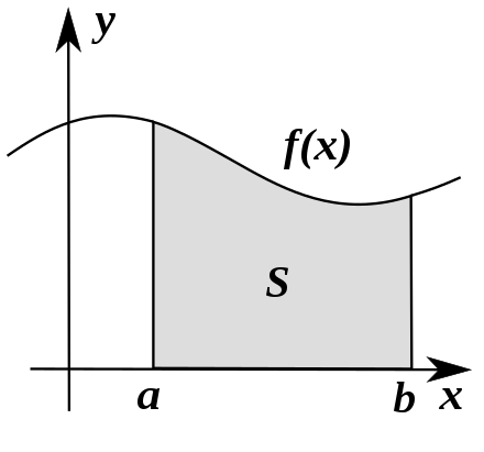
Numerical integration is used to calculate a numerical approximation for the value {\displaystyle S}S, the area under the curve defined by {\displaystyle f(x)}f(x).

1 Reasons for numerical integration
2 History
3 Methods for one-dimensional integrals
4 Multidimensional integrals
5 Connection with differential equations
6 See also

1 Reasons for numerical integration

There are several reasons for carrying out numerical integration, as opposed to analytical integration by finding the antiderivative:

The integrand f(x) may be known only at certain points, such as obtained by sampling. Some embedded systems and other computer applications may need numerical integration for this reason.
A formula for the integrand may be known, but it may be difficult or impossible to find an antiderivative that is an elementary function. An example of such an integrand is f(x) = exp(−x2), the antiderivative of which (the error function, times a constant) cannot be written in elementary form.
See also: nonelementary integral
It may be possible to find an antiderivative symbolically, but it may be easier to compute a numerical approximation than to compute the antiderivative. That may be the case if the antiderivative is given as an infinite series or product, or if its evaluation requires a special function that is not available.