卷积神经网络（卷积+池化+全连接）

一、使用边缘检测来说明卷积操作

卷积是操作是卷积神经网络的基本组成之一。

1.1 卷积是如何操作的？

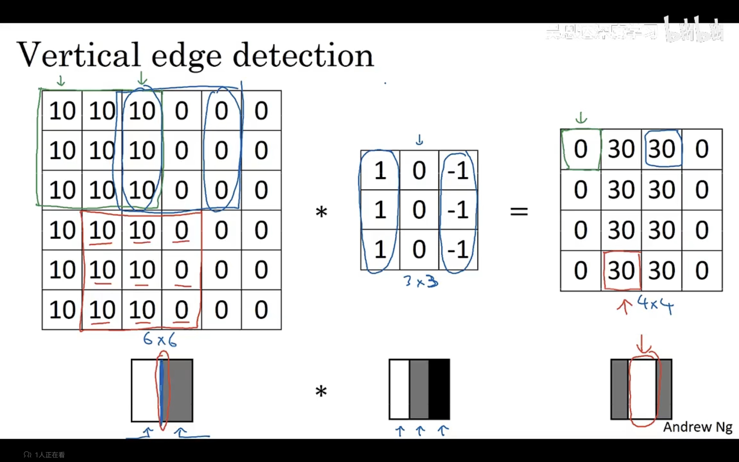
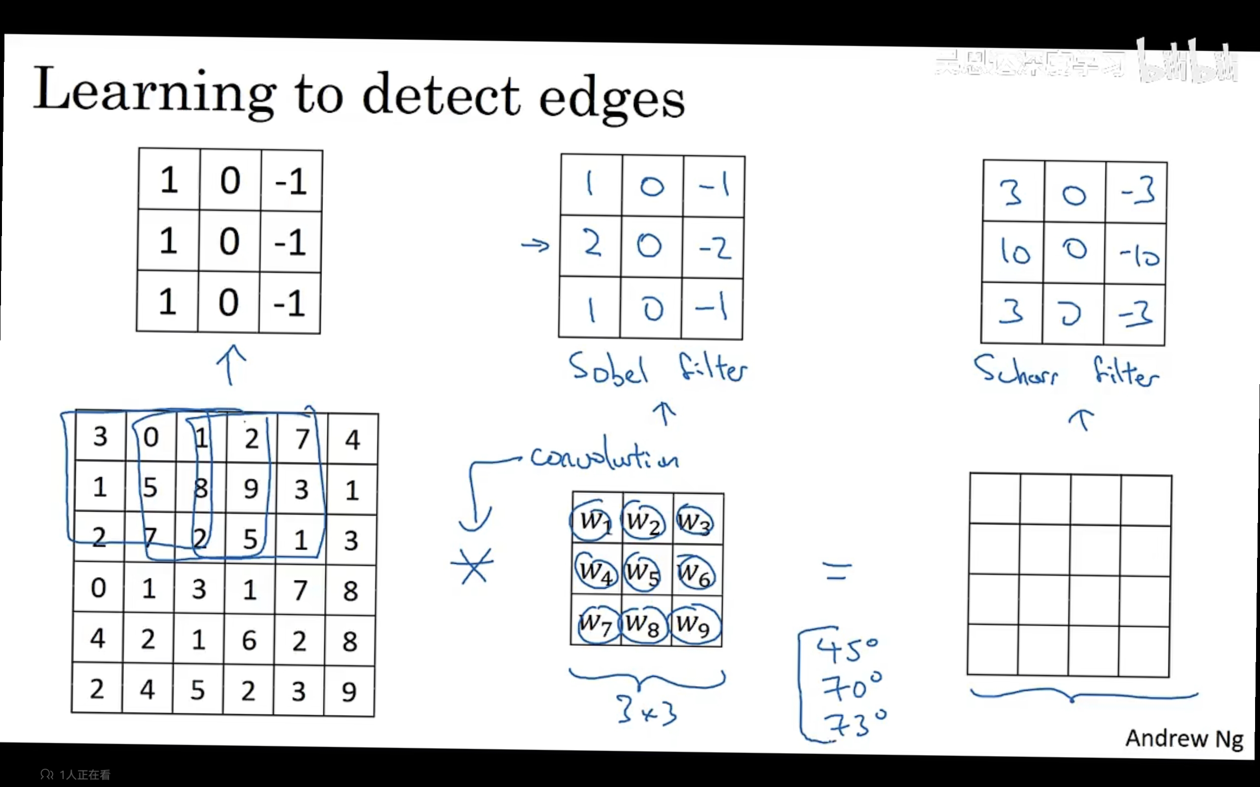
垂直边缘探测器，示例如下：

计算4×4过滤后图像的左上角区域，是将过滤器的大小3×3粘贴到原始输入图像的3×3区域的顶部，粘贴之后将同样位置上的数字相乘再想加，得到一个总和，就会得到过滤之后4×4左上角的数字。过滤后矩阵的下一个值则是将过滤区域平移再次进行计算即可。

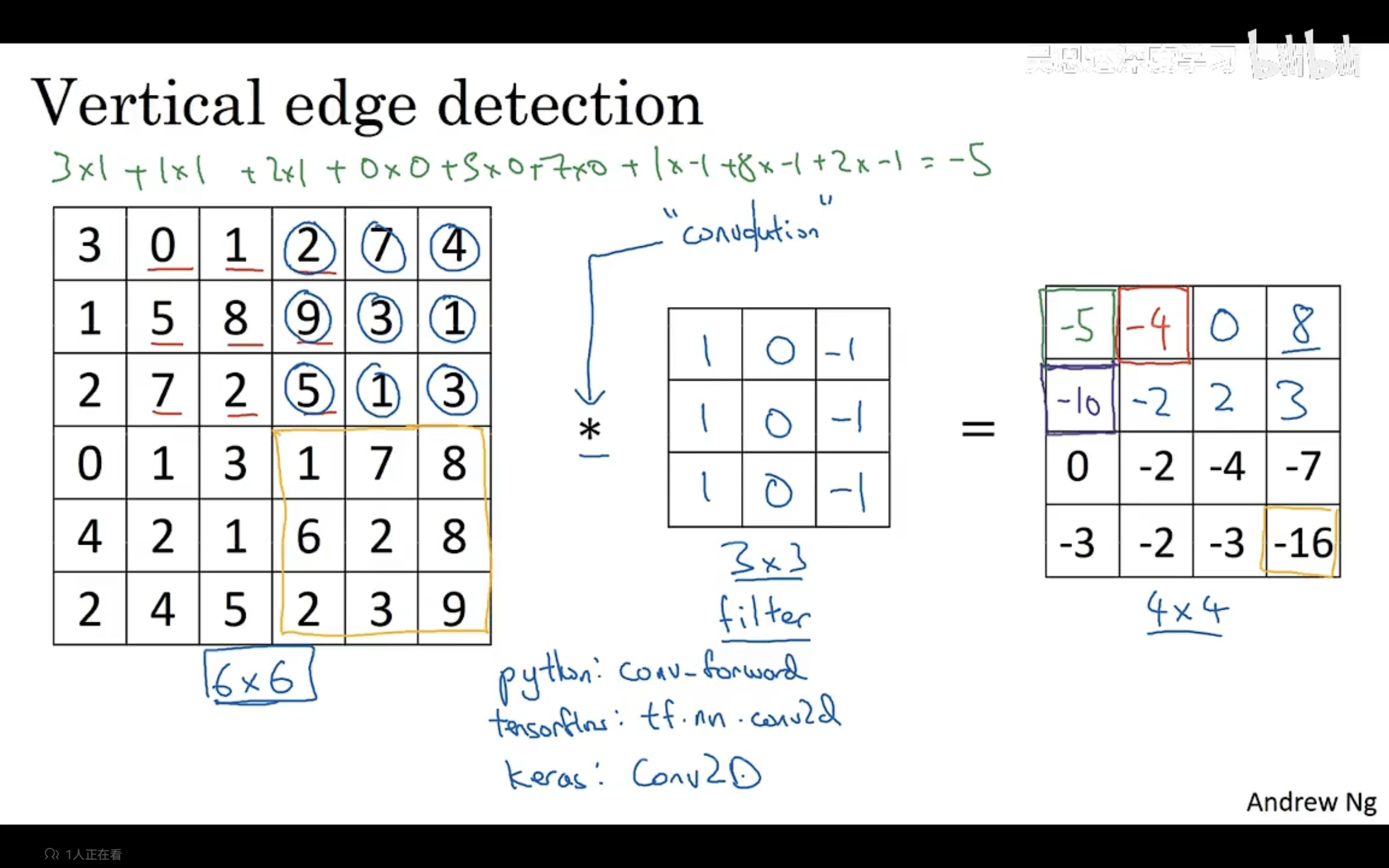
卷积操作提供了一种方便的方法来指定如何在图像中找到垂直边缘。

1.2 更多边缘检测内容

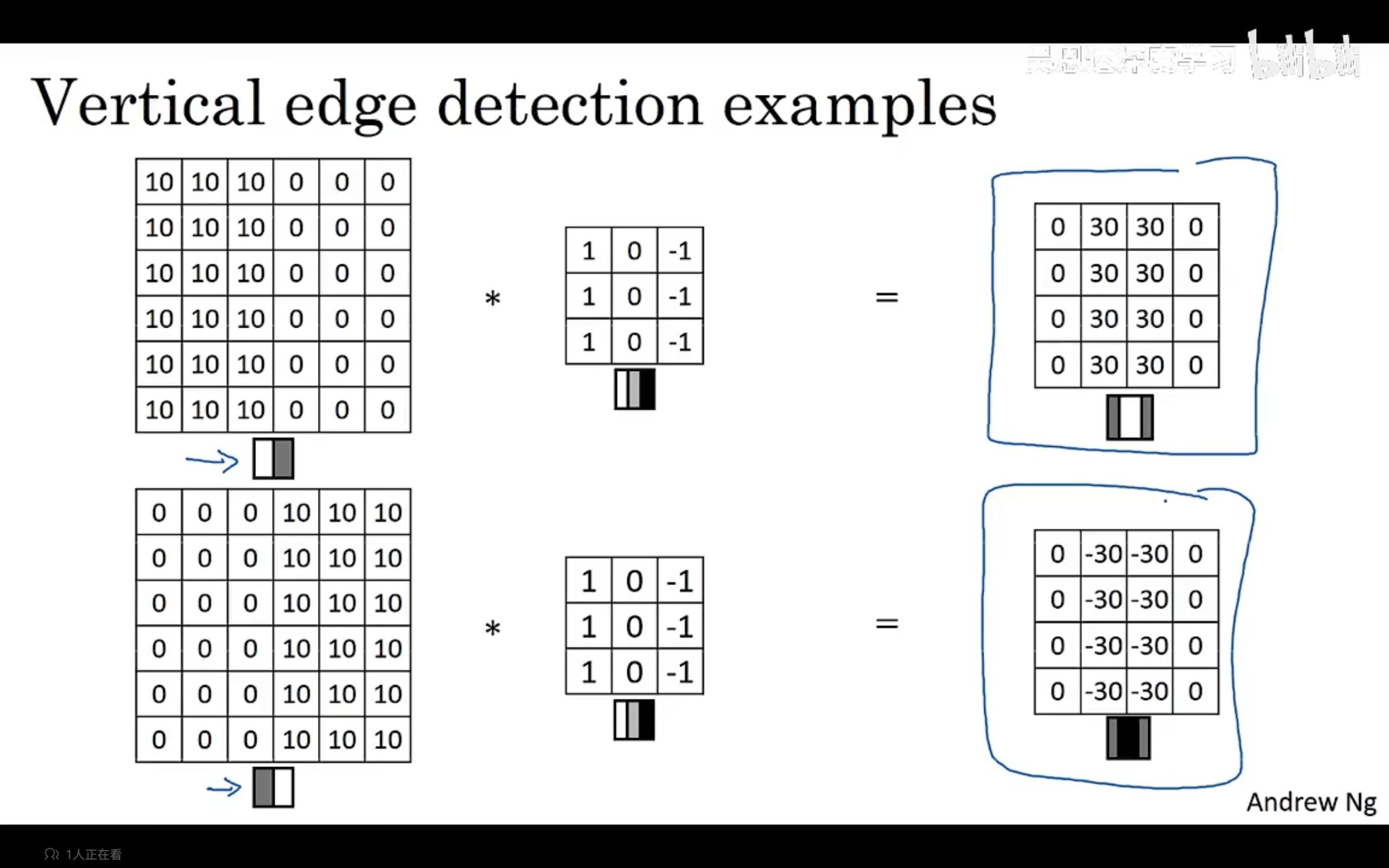
示例中的滤波器区分了从亮到暗和从暗到亮的边缘。

3×3滤波器也可以进行水平边缘检测，将滤波器修改为表示上层较亮，下层较暗对示例进行水平边缘检测如下：

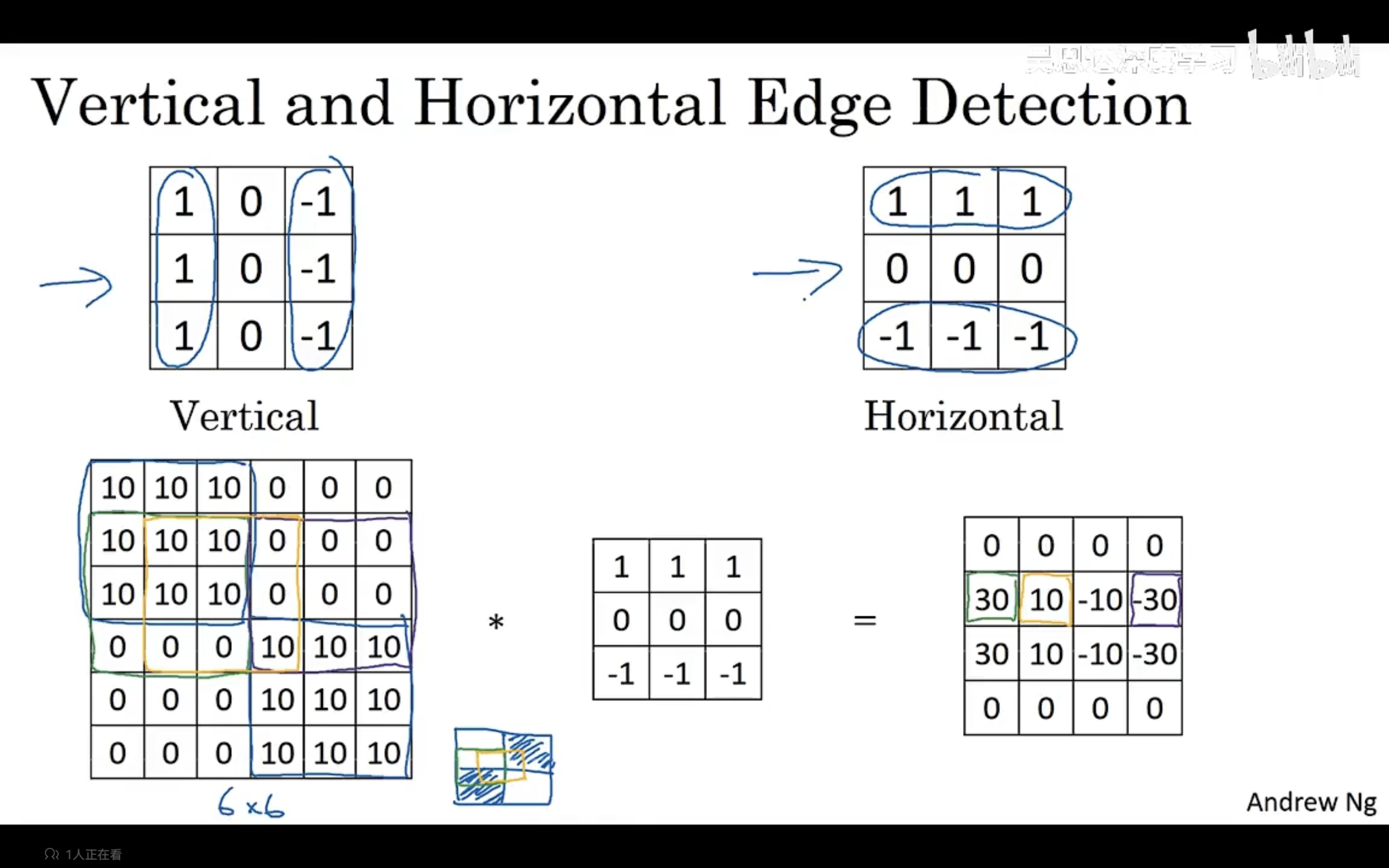
不同的滤波器允许我们找到水平边缘或者垂直边缘。上行中间的被称为索贝尔滤波器（更加重视中间像素），我们也可以将滤波器中的数字作为9个参数进行训练学习，使用反向传播去学习。

二、Padding(图像填充)

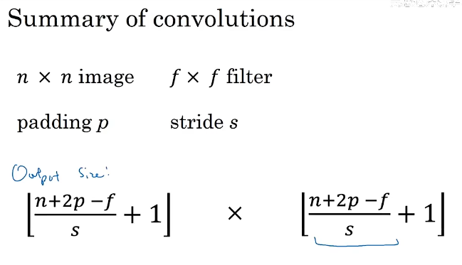
如果原图像是n×n的矩阵，滤波器为f×f的矩阵，那么卷积之后得到的将会是n-f+1×n-f+1的新的图像矩阵。

另外卷积的操作会有两个缺点，第一个是每次卷积以后图像会变小，第二个是边缘的像素点被使用的次数比中间元素被使用的频率少的多，丢弃了图像边缘的大量信息。为了解决这两个问题，我们可以在对图像进行卷积之前先对图像进行填充，加上一个边框，卷积之后保留原始图像的大小。

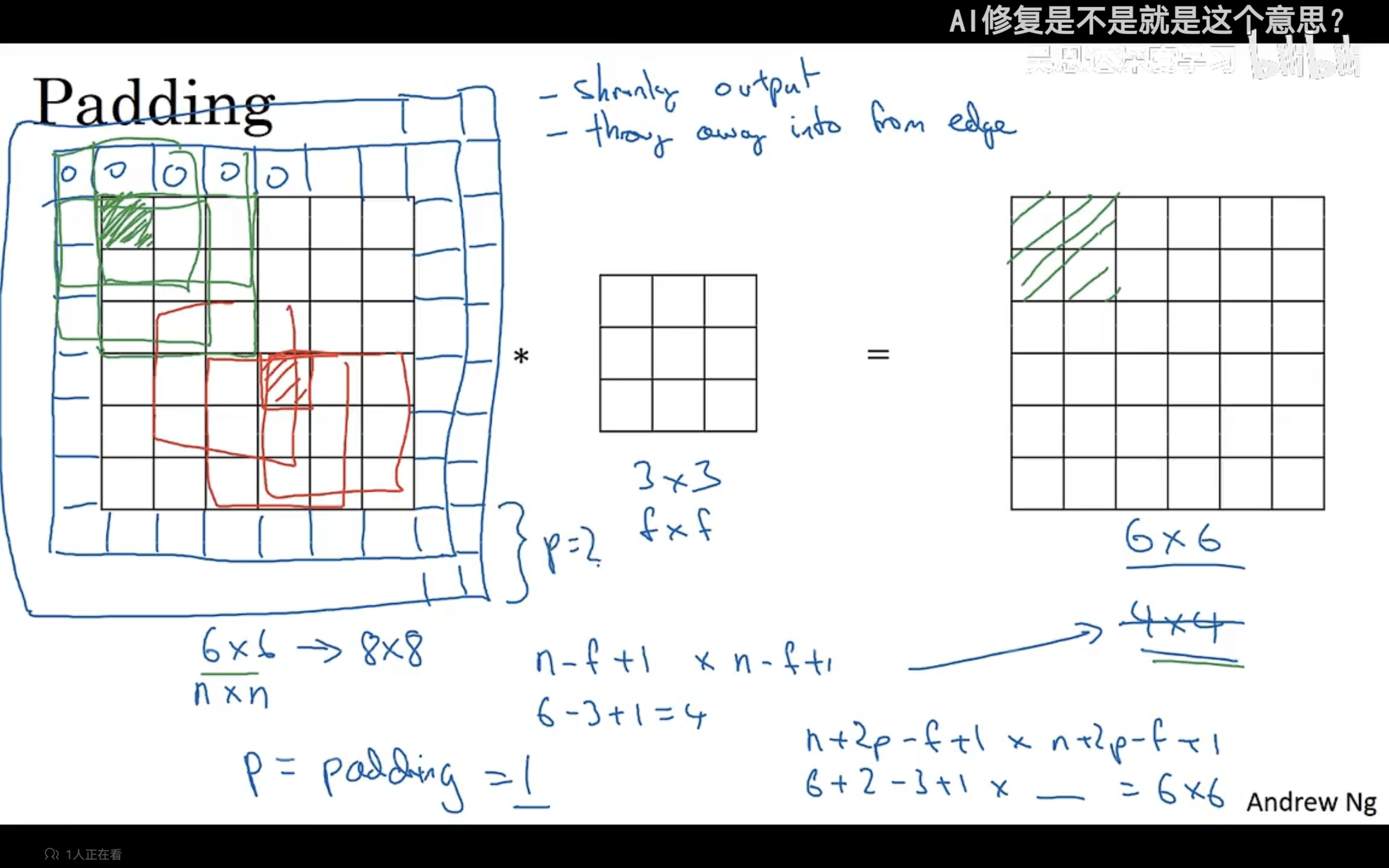
这时候如果我们为图像每个边添加p像素，卷积之后的图像矩阵大小就为（n+2p-f+1）×（n+2p-f+1）。

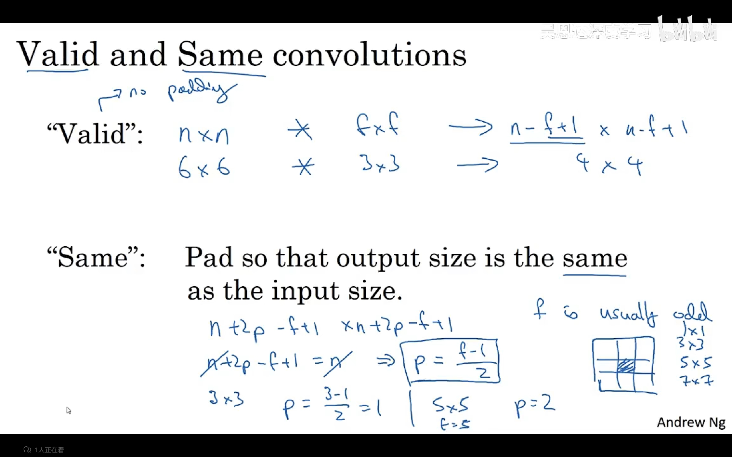
具体填充多少像素呢？最基本的有两种填充方式，第一种是无填充，第二种是填充p，使得填充之后的图像经过卷积后得到的图像大小与原图像大小一致。

计算机视觉中，f的大小几乎总是奇数，可能有两个原因，f为奇数，在进行填充时能够更方便，对称地进行填充，第二个是奇数有中间位置，在计算机视觉中比较好。

三、卷积步长

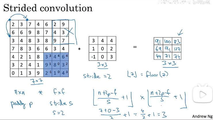
卷积步长指的是我们在卷积过程中进行计算移动时的长度。步长变化之后，我们卷积之后的图像大小也会发生变化，具体变化由下面这个公式来控制：输入的图像大小为nn，滤波器卷积矩阵为ff，填充为p，步长为s，那么卷积之后的图像大小围为：(n+2p-f)/s+1 * (n+2p-f)/s+1.如果这部分的计算结果不为整数，则对它进行向下取整，在计算过程中，如果对图像的卷积部分有一些是悬挂在外面的则不进行计算（滤波器需要完全在图像内获图像加填充区）。

按照惯例在机器学习中，通常不考虑对滤波器进行镜像操作。

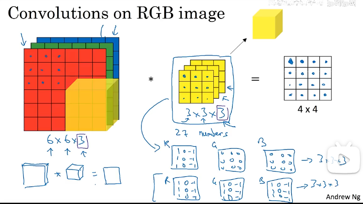
四、三维卷积

当我们对三维数据进行卷积时，滤波器的通道数要与原图像的通道数一致。

卷积的计算方式与二维的是一样的，示例如下：通过设置滤波器中的参数，我们可以检测图像的某一通道的情况或者边缘等图像中的特征。

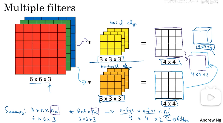
在构建卷积神将网络时，如果我们想同时使用多个滤波器，我们应该如何做？我们可以堆叠输出特征，形成一个三维体积。

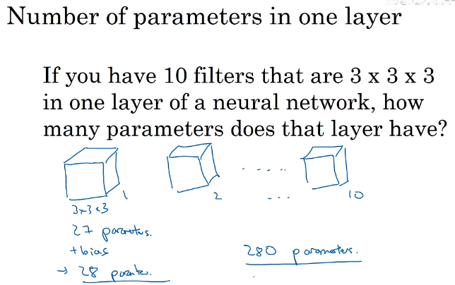
五、单层卷积网络

单层卷积网络包括卷积和接下来的一步：为卷积后的图像添加偏置并进行激活，再将不同的滤波器得到的结果堆叠起来形成单层的卷积网络。其中卷积相当于进行的线性操作（w）

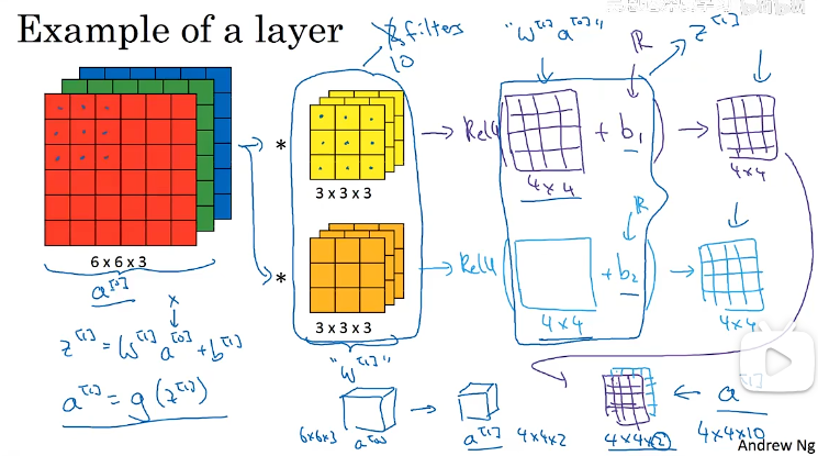
下面的示例中的单层卷积网络有多少个参数呢？一个滤波器有333+1=28个参数，10个滤波器就是280个参数。无论多大的图像，如果想要学习其中的10个特征，那么参数数量都会时280，这样不会导致过拟合。

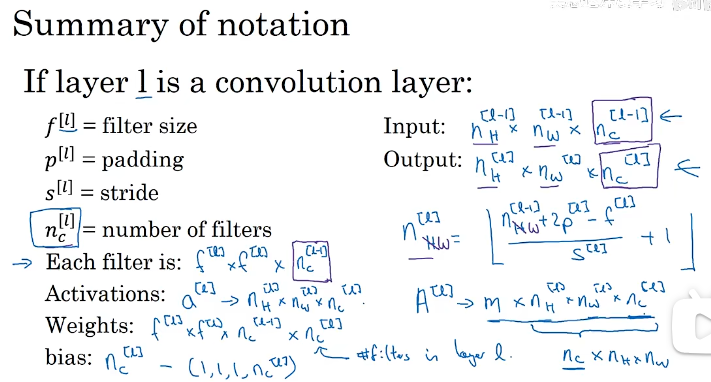
卷积神经网络（类似于普通的神经网络）中两层之间的输入输出大小计算方式如下：

六、简单卷积网络示例

到最后一层卷积结束时，我们可以将最终的特征矩阵展开成一个矢量数据，然后使用逻辑回归或者softmax对数据进行预测。那么再在这整个深层的卷积网络中有很多超参数是需要我们设定的。

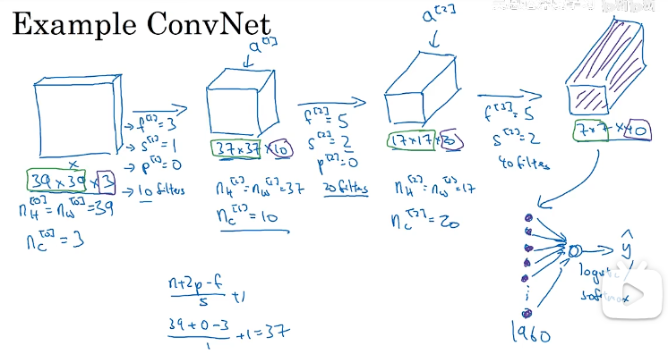
一个典型的卷积网络中通常有三种类型的层：卷积层（conv）、池化层（pool）、全连接层（fc）。

下面是一个简单的卷积神经网络代码示例：

# GRADED FUNCTION: forward_propagation

def forward_propagation(X, parameters):
    """
    Implements the forward propagation for the model:
    CONV2D -> RELU -> MAXPOOL -> CONV2D -> RELU -> MAXPOOL -> FLATTEN -> FULLYCONNECTED
    
    Arguments:
    X -- input dataset placeholder, of shape (input size, number of examples)
    parameters -- python dictionary containing your parameters "W1", "W2"
                  the shapes are given in initialize_parameters

    Returns:
    Z3 -- the output of the last LINEAR unit
    """
    
    # Retrieve the parameters from the dictionary "parameters" 
    W1 = parameters['W1']  # 获取第一个卷积核参数
    W2 = parameters['W2']  # 获取第二个卷积核参数
    
    ### START CODE HERE ###
    # CONV2D: stride of 1, padding 'SAME'
    Z1 = tf.nn.conv2d(X,W1, strides = [1,1,1,1], padding = 'SAME')  # 对输入X进行卷积操作，步长为1，填充方式为'SAME'
    # RELU
    A_temp1 = tf.nn.relu(Z1)  # 对卷积结果Z1进行ReLU激活
    # MAXPOOL: window 8x8, sride 8, padding 'SAME'
    A1 = tf.nn.max_pool(A_temp1, ksize = [1,8,8,1], strides = [1,8,8,1], padding = 'SAME')  # 对激活结果A_temp1进行最大池化，池化窗口为8x8，步长为8，填充方式为'SAME'
    # CONV2D: filters W2, stride 1, padding 'SAME'
    Z2 = tf.nn.conv2d(A1,W2, strides = [1,1,1,1], padding = 'SAME')  # 对池化结果A1进行卷积操作，步长为1，填充方式为'SAME'
    # RELU
    A_temp2 = tf.nn.relu(Z2)  # 对卷积结果Z2进行ReLU激活
    # MAXPOOL: window 4x4, stride 4, padding 'SAME'
    A2 = tf.nn.max_pool(A_temp2, ksize = [1,4,4,1], strides = [1,4,4,1], padding = 'SAME')  # 对激活结果A_temp2进行最大池化，池化窗口为4x4，步长为4，填充方式为'SAME'
    # FLATTEN
    F = tf.contrib.layers.flatten(A2)  # 将池化结果A2展平为一维向量
    # FULLY-CONNECTED without non-linear activation function (not not call softmax).
    # 6 neurons in output layer. Hint: one of the arguments should be "activation_fn=None" 
    Z3 = tf.contrib.layers.fully_connected(F, 6)  # 对展平结果F进行全连接操作，输出层有6个神经元，激活函数为None
    ### END CODE HERE ###

    return Z3  # 返回最后一层的输出结果

模型定义如下：

# GRADED FUNCTION: model

def model(X_train, Y_train, X_test, Y_test, learning_rate=0.009,
          num_epochs=100, minibatch_size=64, print_cost=True):
    """
    实现一个三层 ConvNet：
    CONV2D -> RELU -> MAXPOOL -> CONV2D -> RELU -> MAXPOOL -> FLATTEN -> FULLYCONNECTED
    """
    
    ops.reset_default_graph()                         # 重置默认图，避免重复定义变量
    tf.set_random_seed(1)                             # 固定 TF 随机种子，保证可复现
    seed = 3                                          # NumPy 随机种子
    (m, n_H0, n_W0, n_C0) = X_train.shape             # 训练样本数/高/宽/通道
    n_y = Y_train.shape[1]                            # 类别数（6）
    costs = []                                        # 记录每 epoch 的平均 cost

    # 创建占位符
    ### START CODE HERE ### (1 line)
    X, Y = create_placeholders(n_H0, n_W0, n_C0, n_y)  # 返回 (X, Y) 占位符
    ### END CODE HERE ###

    # 初始化参数
    ### START CODE HERE ### (1 line)
    parameters = initialize_parameters()              # 返回 {"W1":..., "W2":...}
    ### END CODE HERE ###

    # 前向传播
    ### START CODE HERE ### (1 line)
    Z3 = forward_propagation(X, parameters)           # 得到 logits，shape (None, 6)
    ### END CODE HERE ###

    # 计算 cost
    ### START CODE HERE ### (1 line)
    cost = compute_cost(Z3, Y)                        # 返回 softmax-cross-entropy 的平均值
    ### END CODE HERE ###

    # 定义优化器（必须补全！）
    ### START CODE HERE ### (1 line)
    optimizer = tf.train.AdamOptimizer(learning_rate).minimize(cost)  # Adam 优化器
    ### END CODE HERE ###

    # 全局初始化
    init = tf.global_variables_initializer()

    # 启动会话
    with tf.Session() as sess:
        sess.run(init)                                # 初始化所有变量

        # 训练主循环
        for epoch in range(num_epochs):
            minibatch_cost = 0.                       # 当前 epoch 的累计 cost
            num_minibatches = int(m / minibatch_size) # 每个 epoch 的 minibatch 数量
            seed += 1                                 # 保证每个 epoch 的打乱不同
            minibatches = random_mini_batches(X_train, Y_train, minibatch_size, seed)

            for minibatch in minibatches:
                (minibatch_X, minibatch_Y) = minibatch  # 取出当前 minibatch 数据

                # 运行一次反向传播（必须补全！）
                ### START CODE HERE ### (1 line)
                _, temp_cost = sess.run([optimizer, cost],
                                        feed_dict={X: minibatch_X, Y: minibatch_Y})
                ### END CODE HERE ###

                minibatch_cost += temp_cost / num_minibatches  # 累加平均 cost

            # 打印 cost
            if print_cost and epoch % 5 == 0:
                print("Cost after epoch %i: %f" % (epoch, minibatch_cost))
            if print_cost and epoch % 1 == 0:
                costs.append(minibatch_cost)

        # 绘制 cost 曲线
        plt.plot(np.squeeze(costs))
        plt.ylabel('cost')
        plt.xlabel('iterations (per tens)')
        plt.title("Learning rate =" + str(learning_rate))
        plt.show()

        # 计算准确率
        predict_op = tf.argmax(Z3, 1)                    # 预测类别
        correct_prediction = tf.equal(predict_op, tf.argmax(Y, 1))
        accuracy = tf.reduce_mean(tf.cast(correct_prediction, "float"))

        # 评估训练集与测试集
        train_accuracy = accuracy.eval({X: X_train, Y: Y_train})
        test_accuracy  = accuracy.eval({X: X_test,  Y: Y_test})
        print("Train Accuracy:", train_accuracy)
        print("Test Accuracy:", test_accuracy)

        return train_accuracy, test_accuracy, parameters

七、池化层

卷积通常使用池化层来减小表示的大小，来加速计算，使检测到的特征更加稳定。

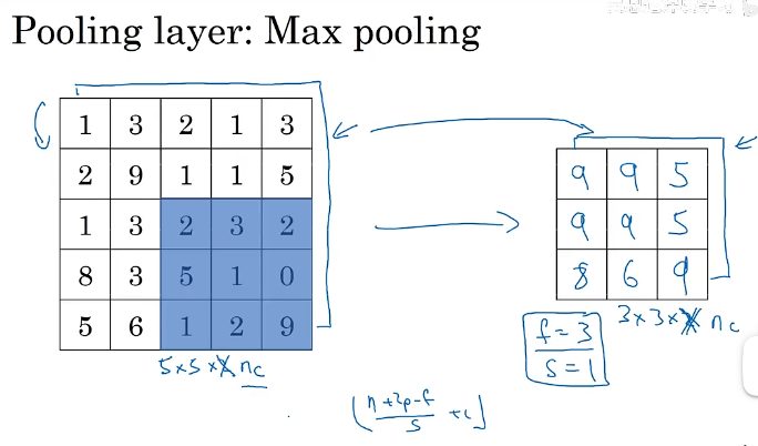
7.1 最大池化

最大池化的池化输出为22，对于输入的图像，我们可以将其分成几个部分，对应22中每个单元将是对应阴影区域的最大值。最大池化超参数（大小为2*2，步长为2）。

使用其他参数的池化示例：这里需要注意的是：池化之后的图像大小的计算方式和卷积是一致的。

7.2 平均池化

不同之处在于：不是在每个滤波器内取最大值，而是取平均值。

池化的超参数有滤波器的大小、步长、最大池化还是平均值池化。最大池化通常不使用任何填充。

八、更加复杂的卷积神经网络

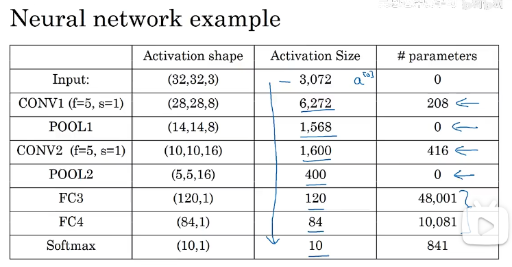
下面这个示例中包含了两个卷积层、两个池化层、三个全连接层。

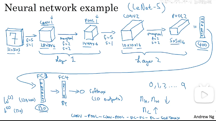
下面的表格中展示每一层的参数大小，可以里看到池化层是没有要学习的参数，卷积层的参数较少，而更多的参数则是分布在全连接层。

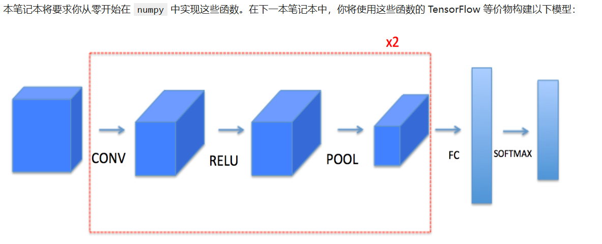
8.1 下面实现神经网络的基本模块。

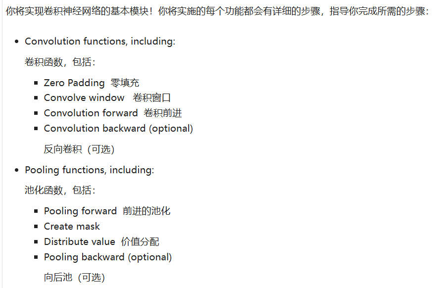
8.2 零填充（Zero-Padding）

它允许你使用 CONV 图层，而不一定缩小体积的高度和宽度。这对于构建更深层的网络很重要，否则层越深，高度和宽度就会变小。一个重要的特例是“相同”卷积，其中一层后高度/宽度完全保持不变。它帮助我们将更多信息保留在图像的边界。没有填充，下一层很少有值会被像素作为图像边缘的影响。

# GRADED FUNCTION: zero_pad

def zero_pad(X, pad):
    """
    Pad with zeros all images of the dataset X. The padding is applied to the height and width of an image, 
    as illustrated in Figure 1.
    
    Argument:
    X -- python numpy array of shape (m, n_H, n_W, n_C) representing a batch of m images
    pad -- integer, amount of padding around each image on vertical and horizontal dimensions
    
    Returns:
    X_pad -- padded image of shape (m, n_H + 2*pad, n_W + 2*pad, n_C)
    """
    
    ### START CODE HERE ### (≈ 1 line)
    X_pad = np.pad(X, ((0, 0), (pad, pad), (pad, pad), (0, 0)), 'constant', constant_values=0)   # 在X的维度上面左右或者上下进行填充，其余不填充
    ### END CODE HERE ###
    
    return X_pad

8.3 单步卷积操作

# GRADED FUNCTION: conv_single_step

def conv_single_step(a_slice_prev, W, b):
    """
    Apply one filter defined by parameters W on a single slice (a_slice_prev) of the output activation 
    of the previous layer.
    
    Arguments:
    a_slice_prev -- slice of input data of shape (f, f, n_C_prev)
    W -- Weight parameters contained in a window - matrix of shape (f, f, n_C_prev)
    b -- Bias parameters contained in a window - matrix of shape (1, 1, 1)
    
    Returns:
    Z -- a scalar value, result of convolving the sliding window (W, b) on a slice x of the input data
    """

    ### START CODE HERE ### (≈ 2 lines of code)
    # Element-wise product between a_slice and W. Add bias.
    A = np.multiply(a_slice_prev,W)+b   # 卷积区域逐元素相乘
    # Sum over all entries of the volume s
    Z = np.sum(A)  # 再相加
    ### END CODE HERE ###

    return Z

8.4 卷积向前传播

# GRADED FUNCTION: conv_forward

def conv_forward(A_prev, W, b, hparameters):
    """
    Implements the forward propagation for a convolution function
    
    Arguments:
    A_prev -- output activations of the previous layer, numpy array of shape (m, n_H_prev, n_W_prev, n_C_prev)
    W -- Weights, numpy array of shape (f, f, n_C_prev, n_C)
    b -- Biases, numpy array of shape (1, 1, 1, n_C)
    hparameters -- python dictionary containing "stride" and "pad"
        
    Returns:
    Z -- conv output, numpy array of shape (m, n_H, n_W, n_C)
    cache -- cache of values needed for the conv_backward() function
    """
    
    ### START CODE HERE ###
    # Retrieve dimensions from A_prev's shape (≈1 line)  
    (m, n_H_prev, n_W_prev, n_C_prev) = A_prev.shape          # 获取输入样本数、高、宽、通道数
    
    # Retrieve dimensions from W's shape (≈1 line)
    (f, f, n_C_prev, n_C) = W.shape                           # 获取滤波器尺寸、输入/输出通道数
    
    # Retrieve information from "hparameters" (≈2 lines)
    stride = hparameters['stride']                            # 读取步长
    pad    = hparameters['pad']                               # 读取填充量
    
    # Compute the dimensions of the CONV output volume using the formula given above. Hint: use int() to floor. (≈2 lines)
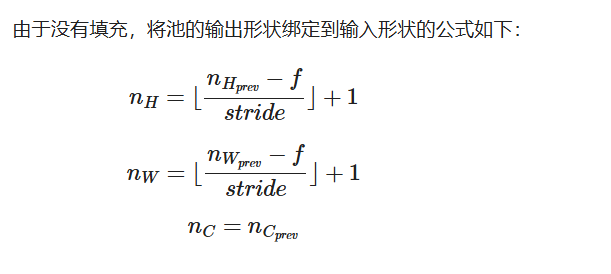
    n_H = int((n_H_prev + 2 * pad - f) / stride) + 1        # 计算输出特征图高度
    n_W = int((n_W_prev + 2 * pad - f) / stride) + 1        # 计算输出特征图宽度
    
    # Initialize the output volume Z with zeros. (≈1 line)
    Z = np.zeros((m, n_H, n_W, n_C))                          # 初始化输出张量
    
    # Create A_prev_pad by padding A_prev
    A_prev_pad = zero_pad(A_prev, pad)                        # 对输入进行零填充
    
    # loop over the batch of training examples
    for i in range(m):                                        # 遍历每个样本
        # Select ith training example's padded activation
        a_prev_pad = A_prev_pad[i]                            # 取出第 i 个样本的填充后特征图
        # loop over vertical axis of the output volume
        for h in range(n_H):                                  # 遍历输出垂直方向
            # loop over horizontal axis of the output volume
            for w in range(n_W):                              # 遍历输出水平方向
                # loop over channels (= #filters) of the output volume
                for c in range(n_C):                          # 遍历每个输出通道（滤波器）
                    
                    # Find the corners of the current "slice" (≈4 lines)
                    vert_start  = h * stride                  # 计算当前 slice 顶部行号
                    vert_end    = vert_start + f              # 计算当前 slice 底部行号
                    horiz_start = w * stride                  # 计算当前 slice 左侧列号
                    horiz_end   = horiz_start + f             # 计算当前 slice 右侧列号
                    
                    # Use the corners to define the (3D) slice of a_prev_pad (See Hint above the cell). (≈1 line)
                    a_slice = a_prev_pad[vert_start:vert_end, horiz_start:horiz_end, :]  # 截取 3D 切片
                    
                    # Convolve the (3D) slice with the correct filter W and bias b, to get back one output neuron. (≈1 line)
                    Z[i, h, w, c] = conv_single_step(a_slice, W[..., c], b[..., c])     # 单步卷积运算
    ### END CODE HERE ###
    
    # Making sure your output shape is correct
    assert(Z.shape == (m, n_H, n_W, n_C))
    
    # Save information in "cache" for the backprop
    cache = (A_prev, W, b, hparameters)
    
    return Z, cache

8.5 池化

这些池化层没有用于反向传播训练的参数。然而，它们有超参数，如窗口大小 f。这指定了你要计算最大或平均值的 fxf 窗口的高度和宽度。

8.5.1 向前池化

# GRADED FUNCTION: pool_forward

def pool_forward(A_prev, hparameters, mode = "max"):
    """
    Implements the forward pass of the pooling layer
    
    Arguments:
    A_prev -- Input data, numpy array of shape (m, n_H_prev, n_W_prev, n_C_prev)
    hparameters -- python dictionary containing "f" and "stride"
    mode -- the pooling mode you would like to use, defined as a string ("max" or "average")
    
    Returns:
    A -- output of the pool layer, a numpy array of shape (m, n_H, n_W, n_C)
    cache -- cache used in the backward pass of the pooling layer, contains the input and hparameters 
    """
    
    # Retrieve dimensions from the input shape
    (m, n_H_prev, n_W_prev, n_C_prev) = A_prev.shape
    
    # Retrieve hyperparameters from "hparameters"
    f = hparameters["f"]
    stride = hparameters["stride"]
    
    # Define the dimensions of the output
    n_H = int(1 + (n_H_prev - f) / stride)
    n_W = int(1 + (n_W_prev - f) / stride)
    n_C = n_C_prev
    
    # Initialize output matrix A
    A = np.zeros((m, n_H, n_W, n_C))              
    
    ### START CODE HERE ###
    # loop over the training examples
    for i in range(m):                                  # 遍历每个样本
        # loop on the vertical axis of the output volume
        for h in range(n_H):                            # 遍历输出高度方向
            # loop on the horizontal axis of the output volume
            for w in range(n_W):                        # 遍历输出宽度方向
                # loop over the channels of the output volume
                for c in range(n_C):                    # 遍历每个通道（深度）
                    
                    # Find the corners of the current "slice" (≈4 lines)
                    vert_start = h * stride             # 当前 slice 顶部行号
                    vert_end = vert_start + f           # 当前 slice 底部行号（不含）
                    horiz_start = w * stride            # 当前 slice 左侧列号
                    horiz_end = horiz_start + f         # 当前 slice 右侧列号（不含）
                    
                    # Use the corners to define the current slice on the ith training example of A_prev, channel c. (≈1 line)
                    a_prev_slice = A_prev[i, vert_start:vert_end, horiz_start:horiz_end, c]  # 截取 2D 切片
                    
                    # Compute the pooling operation on the slice. Use an if statement to differentiate the modes. Use np.max/np.mean.
                    if mode == "max":                   # 最大池化
                        A[i, h, w, c] = np.max(a_prev_slice)
                    elif mode == "average":             # 平均池化
                        A[i, h, w, c] = np.mean(a_prev_slice)
    ### END CODE HERE ###
    
    # Store the input and hparameters in "cache" for pool_backward()
    cache = (A_prev, hparameters)
    
    # Making sure your output shape is correct
    assert(A.shape == (m, n_H, n_W, n_C))
    
    return A, cache

8.6 卷积层的反向传播

def conv_backward(dZ, cache):
    """
    Implement the backward propagation for a convolution function
    
    Arguments:
    dZ -- gradient of the cost with respect to the output of the conv layer (Z), numpy array of shape (m, n_H, n_W, n_C)
    cache -- cache of values needed for the conv_backward(), output of conv_forward()
    
    Returns:
    dA_prev -- gradient of the cost with respect to the input of the conv layer (A_prev),
               numpy array of shape (m, n_H_prev, n_W_prev, n_C_prev)
    dW -- gradient of the cost with respect to the weights of the conv layer (W)
          numpy array of shape (f, f, n_C_prev, n_C)
    db -- gradient of the cost with respect to the biases of the conv layer (b)
          numpy array of shape (1, 1, 1, n_C)
    """
    
    ### START CODE HERE ###
    # Retrieve information from "cache"
    (A_prev, W, b, hparameters) = cache           # 从 cache 取出前向传播保存的值
    
    # Retrieve dimensions from A_prev's shape
    (m, n_H_prev, n_W_prev, n_C_prev) = A_prev.shape   # 输入样本数、高、宽、通道
    
    # Retrieve dimensions from W's shape
    (f, f, n_C_prev, n_C) = W.shape                    # 滤波器尺寸与输入/输出通道数
    
    # Retrieve information from "hparameters"
    stride = hparameters['stride']                     # 步长
    pad = hparameters['pad']                           # 填充量
    
    # Retrieve dimensions from dZ's shape
    (m, n_H, n_W, n_C) = dZ.shape                      # 输出梯度维度
    
    # Initialize dA_prev, dW, db with the correct shapes
    dA_prev = np.zeros((m, n_H_prev, n_W_prev, n_C_prev))  # 输入梯度初始化
    dW = np.zeros((f, f, n_C_prev, n_C))                   # 权重梯度初始化
    db = np.zeros((1, 1, 1, n_C))                          # 偏置梯度初始化
    
    # Pad A_prev and dA_prev
    A_prev_pad = zero_pad(A_prev, pad)                     # 前向输入填充
    dA_prev_pad = zero_pad(dA_prev, pad)                   # 输入梯度填充
    
    # loop over the training examples
    for i in range(m):                                     # 遍历每个样本
        # select ith training example from A_prev_pad and dA_prev_pad
        a_prev_pad = A_prev_pad[i]                         # 当前样本的填充特征图
        da_prev_pad = dA_prev_pad[i]                       # 当前样本的输入梯度
        
        # loop over vertical axis of the output volume
        for h in range(n_H):                               # 遍历输出高度
            # loop over horizontal axis of the output volume
            for w in range(n_W):                           # 遍历输出宽度
                # loop over the channels of the output volume
                for c in range(n_C):                       # 遍历输出通道（滤波器）
                    
                    # Find the corners of the current "slice"
                    vert_start = h * stride                # 切片顶部行号
                    vert_end = vert_start + f              # 切片底部行号（不含）
                    horiz_start = w * stride               # 切片左侧列号
                    horiz_end = horiz_start + f            # 切片右侧列号（不含）
                    
                    # Use the corners to define the slice from a_prev_pad
                    a_slice = a_prev_pad[vert_start:vert_end, horiz_start:horiz_end, :]  # 截取 3D 切片
                    
                    # Update gradients for the window and the filter's parameters using the code formulas given above
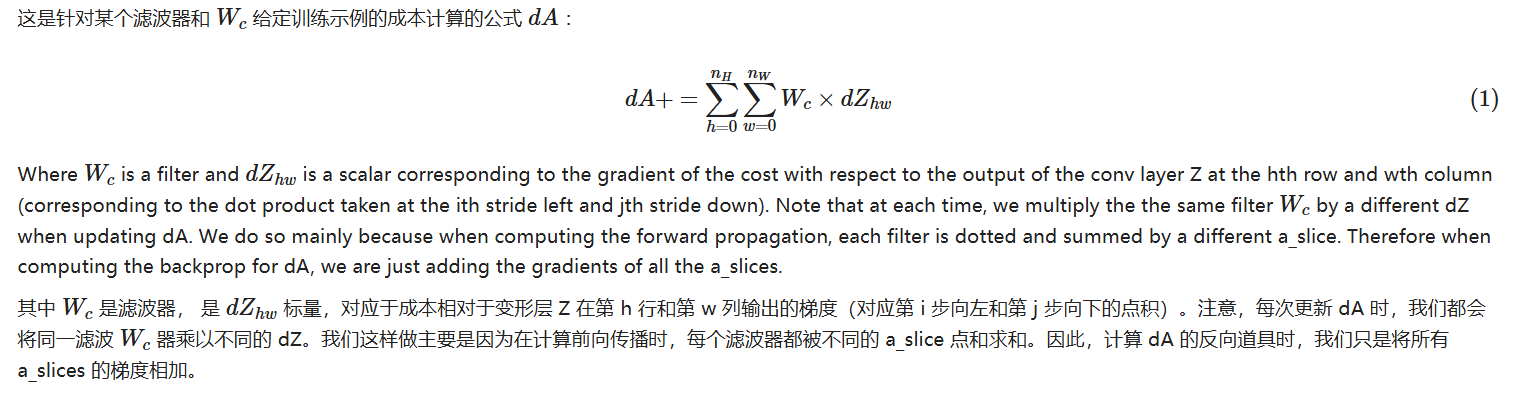
                    da_prev_pad[vert_start:vert_end, horiz_start:horiz_end, :] += W[:, :, :, c] * dZ[i, h, w, c]  # 累加输入梯度
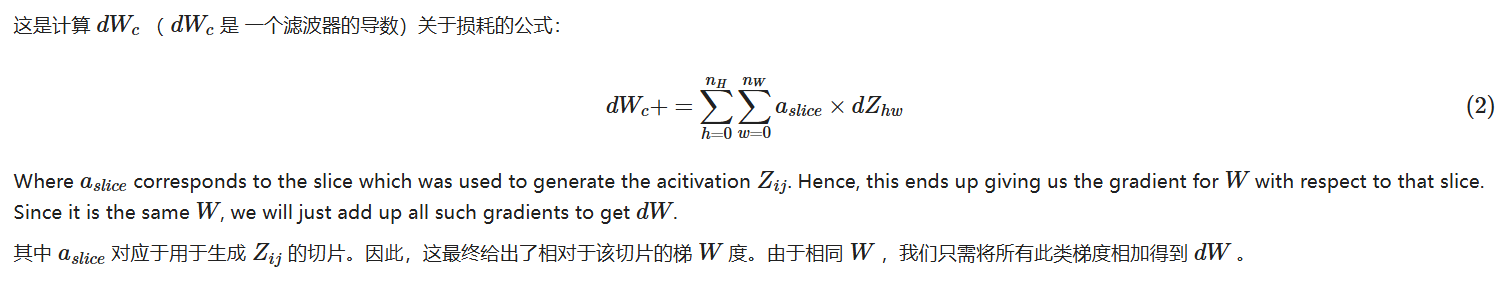
                    dW[:, :, :, c] += a_slice * dZ[i, h, w, c]                           # 累加权重梯度
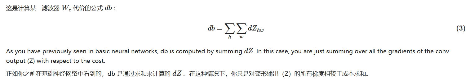
                    db[:, :, :, c] += dZ[i, h, w, c]                                     # 累加偏置梯度
        
        # Set the ith training example's dA_prev to the unpadded da_prev_pad (Hint: use X[pad:-pad, pad:-pad, :])
        dA_prev[i, :, :, :] = da_prev_pad[pad:-pad, pad:-pad, :]  # 去掉填充部分，写回原始尺寸
    
    ### END CODE HERE ###
    
    # Making sure your output shape is correct
    assert(dA_prev.shape == (m, n_H_prev, n_W_prev, n_C_prev))
    
    return dA_prev, dW, db

8.7 池化层的反向传播

8.7.1 最大池的反向传播

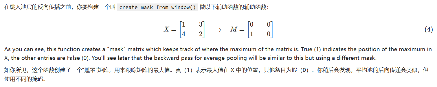
def create_mask_from_window(x):
    """
    Creates a mask from an input matrix x, to identify the max entry of x.
    
    Arguments:
    x -- Array of shape (f, f)
    
    Returns:
    mask -- Array of the same shape as window, contains a True at the position corresponding to the max entry of x.
    """
    
    ### START CODE HERE ### (≈1 line)
    mask = (x == np.max(x))  # 生成布尔掩码：最大值位置为 True，其余为 False
    ### END CODE HERE ###
    
    return mask              # 返回与 x 同形状的掩码矩阵

我们为什么要记录最大值的位置？因为这是最终影响产出和成本的投入值。反向推进计算的是相对于成本的梯度，所以任何影响最终成本的因素都应该有非零梯度。因此，反向推进会将梯度“传播”回这个影响成本的特定输入值。

8.7.2 平均值池化的反向传播

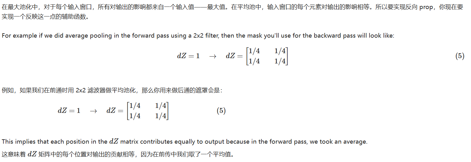
def distribute_value(dz, shape):
    """
    Distributes the input value in the matrix of dimension shape
    
    Arguments:
    dz -- input scalar
    shape -- the shape (n_H, n_W) of the output matrix for which we want to distribute the value of dz
    
    Returns:
    a -- Array of size (n_H, n_W) for which we distributed the value of dz
    """
    
    ### START CODE HERE ###
    # Retrieve dimensions from shape (≈1 line)
    (n_H, n_W) = shape                         # 获取输出矩阵的高和宽
    
    # Compute the value to distribute on the matrix (≈1 line)
    average = dz / (n_H * n_W)                 # 每个元素分摊到的值
    
    # Create a matrix where every entry is the "average" value (≈1 line)
    a = np.ones(shape) * average               # 生成全为 average 的矩阵
    ### END CODE HERE ###
    
    return a                                   # 返回分布后的矩阵

8.7.3 汇总池化的反向传播

def pool_backward(dA, cache, mode = "max"):
    """
    Implements the backward pass of the pooling layer
    
    Arguments:
    dA -- gradient of cost with respect to the output of the pooling layer, same shape as A
    cache -- cache output from the forward pass of the pooling layer, contains the layer's input and hparameters 
    mode -- the pooling mode you would like to use, defined as a string ("max" or "average")
    
    Returns:
    dA_prev -- gradient of cost with respect to the input of the pooling layer, same shape as A_prev
    """
    
    ### START CODE HERE ###

    # Retrieve information from cache (≈1 line)
    (A_prev, hparameters) = cache                    # 取出前向缓存：输入和超参
    
    # Retrieve hyperparameters from "hparameters" (≈2 lines)
    f      = hparameters['f']                        # 池化窗口大小
    stride = hparameters['stride']                   # 步长
    
    # Retrieve dimensions from A_prev's shape and dA's shape (≈2 lines)
    m, n_H_prev, n_W_prev, n_C_prev = A_prev.shape   # 输入维度
    m, n_H, n_W, n_C = dA.shape                      # 输出梯度维度
    
    # Initialize dA_prev with zeros (≈1 line)
    dA_prev = np.zeros_like(A_prev)                  # 初始化输入梯度
    
    # loop over the training examples
    for i in range(m):                                 # 遍历每个样本
        # select training example from A_prev (≈1 line)
        a_prev = A_prev[i]                             # 当前样本特征图
        
        # loop on the vertical axis
        for h in range(n_H):                           # 遍历输出高度
            # loop on the horizontal axis
            for w in range(n_W):                       # 遍历输出宽度
                # loop over the channels (depth)
                for c in range(n_C):                   # 遍历每个通道
                    
                    # Find the corners of the current "slice" (≈4 lines)
                    vert_start  = h * stride           # 切片顶部
                    vert_end    = vert_start + f       # 切片底部（不含）
                    horiz_start = w * stride           # 切片左侧
                    horiz_end   = horiz_start + f      # 切片右侧（不含）
                    
                    # Compute the backward propagation in both modes.
                    if mode == "max":
                        # Use the corners and "c" to define the current slice from a_prev (≈1 line)
                        a_prev_slice = a_prev[vert_start:vert_end, horiz_start:horiz_end, c]  # 截取 2D 切片
                        
                        # Create the mask from a_prev_slice (≈1 line)
                        mask = create_mask_from_window(a_prev_slice)                          # 最大值掩码
                        
                        # Set dA_prev to be dA_prev + (the mask multiplied by the correct entry of dA) (≈1 line)
                        dA_prev[i, vert_start:vert_end, horiz_start:horiz_end, c] += mask * dA[i, h, w, c]  # 只把梯度给最大值位置
                    
                    elif mode == "average":
                        # Get the value a from dA (≈1 line)
                        da = dA[i, h, w, c]                # 当前梯度值
                        
                        # Define the shape of the filter as fxf (≈1 line)
                        shape = (f, f)                     # 池化窗口形状
                        
                        # Distribute it to get the correct slice of dA_prev. i.e. Add the distributed value of da. (≈1 line)
                        dA_prev[i, vert_start:vert_end, horiz_start:horiz_end, c] += distribute_value(da, shape)  # 平均分配给窗口内所有位置
    
    ### END CODE ###
    
    # Making sure your output shape is correct
    assert(dA_prev.shape == A_prev.shape)
    
    return dA_prev

九、卷积的优势和特点

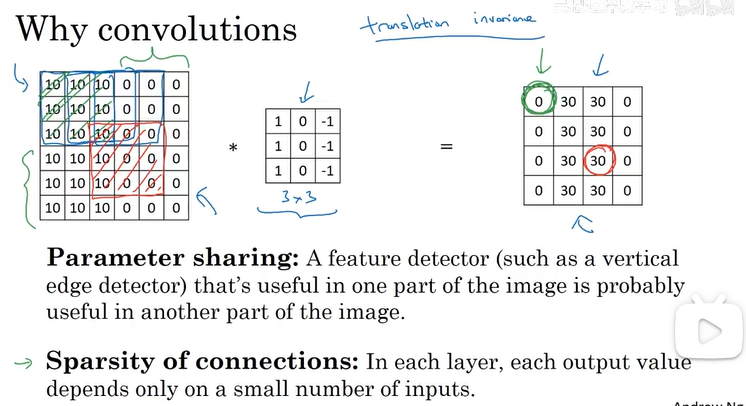
卷积层与全连接层相比第一点优势为：参数共享和连接稀疏。

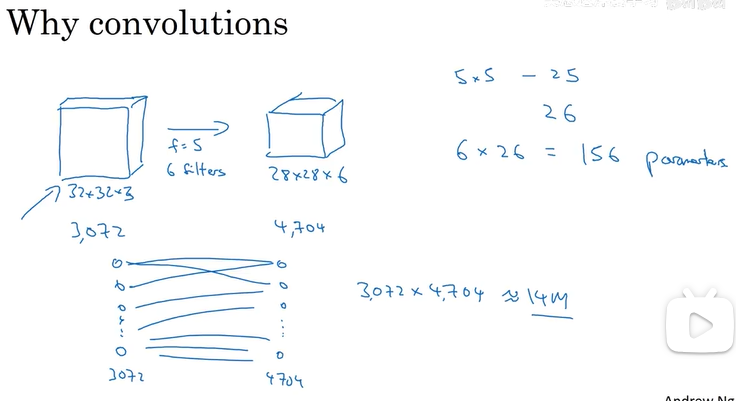
参数共享主要体现在：对于垂直边缘检测器，在图像一部分有用，可能在另一部分也有用，如果已经找出一个滤波器检测垂直边缘，可以在下一个位置应用相同的滤波器。通俗来讲：对于输入数据中较为相似的部分我们可以使用相同的参数来进行计算（我理解的）。连接稀疏：卷积之后的每一个输出可能只来自于输入的某一部分进行卷积得到的，而不是所有的数据。

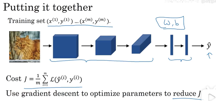
最后给出一个检测猫的卷积网络示例：