Gmsh：三维有限网格生成器

Mineba

已于 2023-12-03 12:02:10 修改

阅读量3k

点赞数 25

分类专栏：科学计算文章标签：学习

于 2023-12-02 22:51:39 首次发布

本文链接：https://blog.csdn.net/qq_74083422/article/details/134758784

版权

科学计算专栏收录该内容

3 篇文章 4 订阅

订阅专栏

网格在科学计算中的重要性

在科学计算中，网格（Grid）是一个离散化的空间描述，将计算领域划分为规则或不规则的小单元。它在科学计算中具有重要性，主要体现在以下方面：

空间离散化：科学计算问题通常涉及对连续空间的离散化，将其划分为有限个网格单元。这样做可以将复杂的数学问题转化为易于计算的离散问题，从而使得计算更加可行和高效。

数值模拟和求解：网格提供了在计算领域内进行数值模拟和求解的基础。通过在网格上建立数学模型和方程，可以将复杂的物理现象转化为离散的计算问题。例如，有限元法和有限差分法等数值方法常常使用网格来近似解析解。

边界条件处理：网格在科学计算中起到了处理边界条件的关键作用。通过将边界位置约束到网格上，可以方便地对边界条件进行定义和处理。这对于模拟物理领域中的流体力学、电磁场等问题尤为重要。

并行计算：在大规模科学计算中，网格的并行划分和处理对于提高计算效率和性能非常关键。通过将网格划分为多个子域并分配给多个计算节点，可以实现并行计算和分布式计算，大大提高计算速度和可扩展性。

网格自适应：在某些情况下，根据问题的复杂性和准确性要求，标准网格可能无法提供足够的解决方案。在这种情况下，网格自适应技术允许根据需要在计算区域中添加或删除网格单元。这种能力对于解决具有局部特征的问题非常重要。

综上所述，网格在科学计算中的重要性不可忽视。它为数值模拟和方程求解提供了基础，处理边界条件，支持并行计算，并能够根据问题的需求进行自适应调整。网格的选择和设计直接影响到科学计算的可靠性、准确性和效率。

Gmsh：三维有限网格生成器

gmsh 是一种开源的三维有限元网格生成器和后处理软件。它具有功能强大和灵活的特点，适用于各种科学计算和工程领域的模拟和分析任务。以下是一些关键特点和功能：

几何建模：gmsh 提供了一个直观的界面，用于创建、修改和操纵复杂的几何模型。用户可以通过手动建模、文件导入、基于CAD软件的集成或编程接口来定义模型。支持包括曲线、曲面、体积等多种几何元素。

网格生成：gmsh 能够生成各种类型的三维有限元网格。用户可以通过选择合适的网格算法、指定划分参数和优化网格质量等方式来控制网格划分。它支持三角形、四边形、四面体、六面体等多种元素类型，并提供自适应网格划分功能。

多物理场模拟：gmsh 支持多种物理场的模拟，包括流体力学、结构力学、电磁场等。用户可以定义边界条件、材料属性、加载条件等，并进行相应的模拟和分析。

后处理功能：gmsh 提供了丰富的后处理功能，用于可视化和分析模拟结果。它支持数据可视化、剖面图、动画等，使用户能够更好地理解和解释模拟结果。

可扩展性：gmsh 是一个开源项目，提供了灵活的接口和插件系统。用户可以使用使用Python ，C，C++，fortran等语言进行自动化建模和网格生成，也可以通过插件来添加新的功能和扩展软件的能力。

总的来说，gmsh 提供了一个强大且易于使用的环境，用于创建、划分和后处理三维有限元网格。它适用于各种科学计算和工程应用，并且具有广泛的用户群体和活跃的社区支持。无论是学术研究还是工程实践，gmsh 都是一个重要的工具。

Gmsh图形界面的安装

这是gmsh的官网：http://gmsh.info

gmshguanwan
选择自己使用的操作系统即可安装，Windows为例，安装后会得到如下文件夹：

wenjianjaigmsh

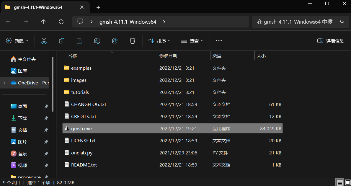
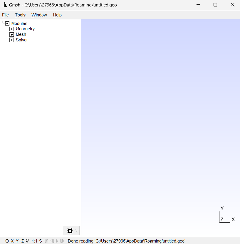
点击exe文件便能打开gmsh的图形窗口：

gmshjiemian

想要查看生成网格效果可以点击文件夹tutorials，里面有各个语言调用gmsh生成网格的实例，还有.geo文件（专门的gmsh几何定义文件，可以构建结几何和生成网格）以t4.geo为例：

// -----------------------------------------------------------------------------
//
//  Gmsh GEO tutorial 4
//
//  Built-in functions, holes in surfaces, annotations, entity colors
//
// -----------------------------------------------------------------------------

// As usual, we start by defining some variables:

cm = 1e-02;
e1 = 4.5 * cm; e2 = 6 * cm / 2; e3 =  5 * cm / 2;
h1 = 5 * cm; h2 = 10 * cm; h3 = 5 * cm; h4 = 2 * cm; h5 = 4.5 * cm;
R1 = 1 * cm; R2 = 1.5 * cm; r = 1 * cm;
Lc1 = 0.01;
Lc2 = 0.003;

// We can use all the usual mathematical functions (note the capitalized first
// letters), plus some useful functions like Hypot(a, b) := Sqrt(a^2 + b^2):

ccos = (-h5*R1 + e2 * Hypot(h5, Hypot(e2, R1))) / (h5^2 + e2^2);
ssin = Sqrt(1 - ccos^2);

// Then we define some points and some lines using these variables:

Point(1) = {-e1-e2, 0    , 0, Lc1}; Point(2) = {-e1-e2, h1   , 0, Lc1};
Point(3) = {-e3-r , h1   , 0, Lc2}; Point(4) = {-e3-r , h1+r , 0, Lc2};
Point(5) = {-e3   , h1+r , 0, Lc2}; Point(6) = {-e3   , h1+h2, 0, Lc1};
Point(7) = { e3   , h1+h2, 0, Lc1}; Point(8) = { e3   , h1+r , 0, Lc2};
Point(9) = { e3+r , h1+r , 0, Lc2}; Point(10)= { e3+r , h1   , 0, Lc2};
Point(11)= { e1+e2, h1   , 0, Lc1}; Point(12)= { e1+e2, 0    , 0, Lc1};
Point(13)= { e2   , 0    , 0, Lc1};

Point(14)= { R1 / ssin, h5+R1*ccos, 0, Lc2};
Point(15)= { 0        , h5        , 0, Lc2};
Point(16)= {-R1 / ssin, h5+R1*ccos, 0, Lc2};
Point(17)= {-e2       , 0.0       , 0, Lc1};

Point(18)= {-R2 , h1+h3   , 0, Lc2}; Point(19)= {-R2 , h1+h3+h4, 0, Lc2};
Point(20)= { 0  , h1+h3+h4, 0, Lc2}; Point(21)= { R2 , h1+h3+h4, 0, Lc2};
Point(22)= { R2 , h1+h3   , 0, Lc2}; Point(23)= { 0  , h1+h3   , 0, Lc2};

Point(24)= { 0, h1+h3+h4+R2, 0, Lc2}; Point(25)= { 0, h1+h3-R2,    0, Lc2};

Line(1)  = {1 , 17};
Line(2)  = {17, 16};

// Gmsh provides other curve primitives than straight lines: splines, B-splines,
// circle arcs, ellipse arcs, etc. Here we define a new circle arc, starting at
// point 14 and ending at point 16, with the circle's center being the point 15:

Circle(3) = {14,15,16};

// Note that, in Gmsh, circle arcs should always be smaller than Pi. The
// OpenCASCADE geometry kernel does not have this limitation.

// We can then define additional lines and circles, as well as a new surface:

Line(4)  = {14, 13}; Line(5)   = {13, 12};   Line(6)    = {12, 11};
Line(7)  = {11, 10}; Circle(8) = {8, 9, 10}; Line(9)    = {8, 7};
Line(10) = {7, 6};   Line(11)  = {6, 5};     Circle(12) = {3, 4, 5};
Line(13) = {3, 2};   Line(14)  = {2, 1};     Line(15)   = {18, 19};
Circle(16) = {21, 20, 24}; Circle(17) = {24, 20, 19};
Circle(18) = {18, 23, 25}; Circle(19) = {25, 23, 22};
Line(20) = {21,22};

Curve Loop(21) = {17, -15, 18, 19, -20, 16};
Plane Surface(22) = {21};

// But we still need to define the exterior surface. Since this surface has a
// hole, its definition now requires two curves loops:

Curve Loop(23) = {11, -12, 13, 14, 1, 2, -3, 4, 5, 6, 7, -8, 9, 10};
Plane Surface(24) = {23, 21};

// As a general rule, if a surface has N holes, it is defined by N+1 curve loops:
// the first loop defines the exterior boundary; the other loops define the
// boundaries of the holes.

// Finally, we can add some comments by embedding a post-processing view
// containing some strings:

View "comments" {
  // Add a text string in window coordinates, 10 pixels from the left and 10
  // pixels from the bottom, using the `StrCat' function to concatenate strings:
  T2(10, -10, 0){ StrCat("Created on ", Today, " with Gmsh") };

  // Add a text string in model coordinates centered at (X,Y,Z) = (0, 0.11, 0):
  T3(0, 0.11, 0, TextAttributes("Align", "Center", "Font", "Helvetica")){
    "Hole"
  };

  // If a string starts with `file://', the rest is interpreted as an image
  // file. For 3D annotations, the size in model coordinates can be specified
  // after a `@' symbol in the form `widthxheight' (if one of `width' or
  // `height' is zero, natural scaling is used; if both are zero, original image
  // dimensions in pixels are used):
  T3(0, 0.09, 0, TextAttributes("Align", "Center")){
    "file://t4_image.png@0.01x0"
  };

  // The 3D orientation of the image can be specified by proving the direction
  // of the bottom and left edge of the image in model space:
  T3(-0.01, 0.09, 0, 0){ "file://t4_image.png@0.01x0,0,0,1,0,1,0" };

  // The image can also be drawn in "billboard" mode, i.e. always parallel to
  // the camera, by using the `#' symbol:
  T3(0, 0.12, 0, TextAttributes("Align", "Center")){
    "file://t4_image.png@0.01x0#"
  };

  // The size of 2D annotations is given directly in pixels:
  T2(350, -7, 0){ "file://t4_image.png@20x0" };
};

// This post-processing view is in the "parsed" format, i.e. it is interpreted
// using the same parser as the `.geo' file. For large post-processing datasets,
// that contain actual field values defined on a mesh, you should use the MSH
// file format instead, which allows to efficiently store continuous or
// discontinuous scalar, vector and tensor fields, or arbitrary polynomial
// order.

// Views and geometrical entities can be made to respond to double-click events,
// here to print some messages to the console:

View[0].DoubleClickedCommand = "Printf('View[0] has been double-clicked!');";
Geometry.DoubleClickedCurveCommand = "Printf('Curve %g has been double-clicked!',
  Geometry.DoubleClickedEntityTag);";

// We can also change the color of some entities:

Color Grey50{ Surface{ 22 }; }
Color Purple{ Surface{ 24 }; }
Color Red{ Curve{ 1:14 }; }
Color Yellow{ Curve{ 15:20 }; }