PCA 主成分分析的代码实现

最新推荐文章于 2025-10-04 13:32:45 发布

qqqweiweiqq

最新推荐文章于 2025-10-04 13:32:45 发布

阅读量152

点赞数

CC 4.0 BY-SA版权

文章标签： python 机器学习 sklearn

本文链接：https://blog.csdn.net/qqqweiweiqq/article/details/129953199

该代码示例展示了如何使用Python的sklearn库进行主成分分析（PCA），首先对数据进行预处理，然后通过PCA降维，最后绘制2D和3D散点图以可视化主要成分，并解释了PCA在数据降维中的作用。

import numpy as np
import pandas as pd
import seaborn as sns
import matplotlib.pyplot as plt
from sklearn.datasets import load_breast_cancer

from sklearn.preprocessing import StandardScaler

from sklearn.decomposition import PCA
from mpl_toolkits import mplot3d

plt.style.use('ggplot')

cancer = load_breast_cancer()

df = pd.DataFrame(data=cancer.data,columns=cancer.feature_names)

x =df.values
print(x.shape)


scaler = StandardScaler()


scaler.fit(x)

x_scaled = scaler.transform(x)

print("x_scaled.shape====",x_scaled.shape)


# ________数据处理阶段完事————————————————————

pca_30 = PCA(n_components=30,random_state=2020)

pca_30.fit(x_scaled)

x_pac_30 =pca_30.transform(x_scaled)


print("np.cumsum====",np.cumsum(pca_30.explained_variance_ratio_*100))

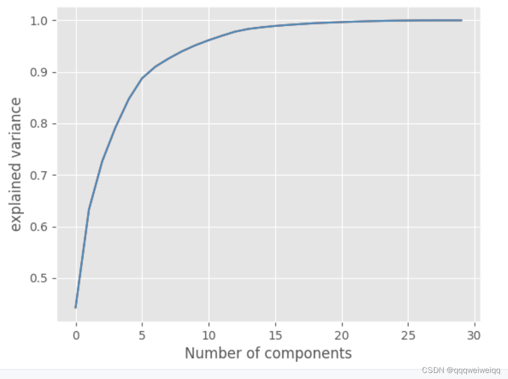
plt.plot(np.cumsum(pca_30.explained_variance_ratio_))

plt.plot(np.cumsum(pca_30.explained_variance_ratio_))

plt.xlabel("Number of components")

plt.ylabel("explained variance")

plt.savefig('elbow_plot',dpi=100)

# 3.d: Apply PCA by setting n_components=2
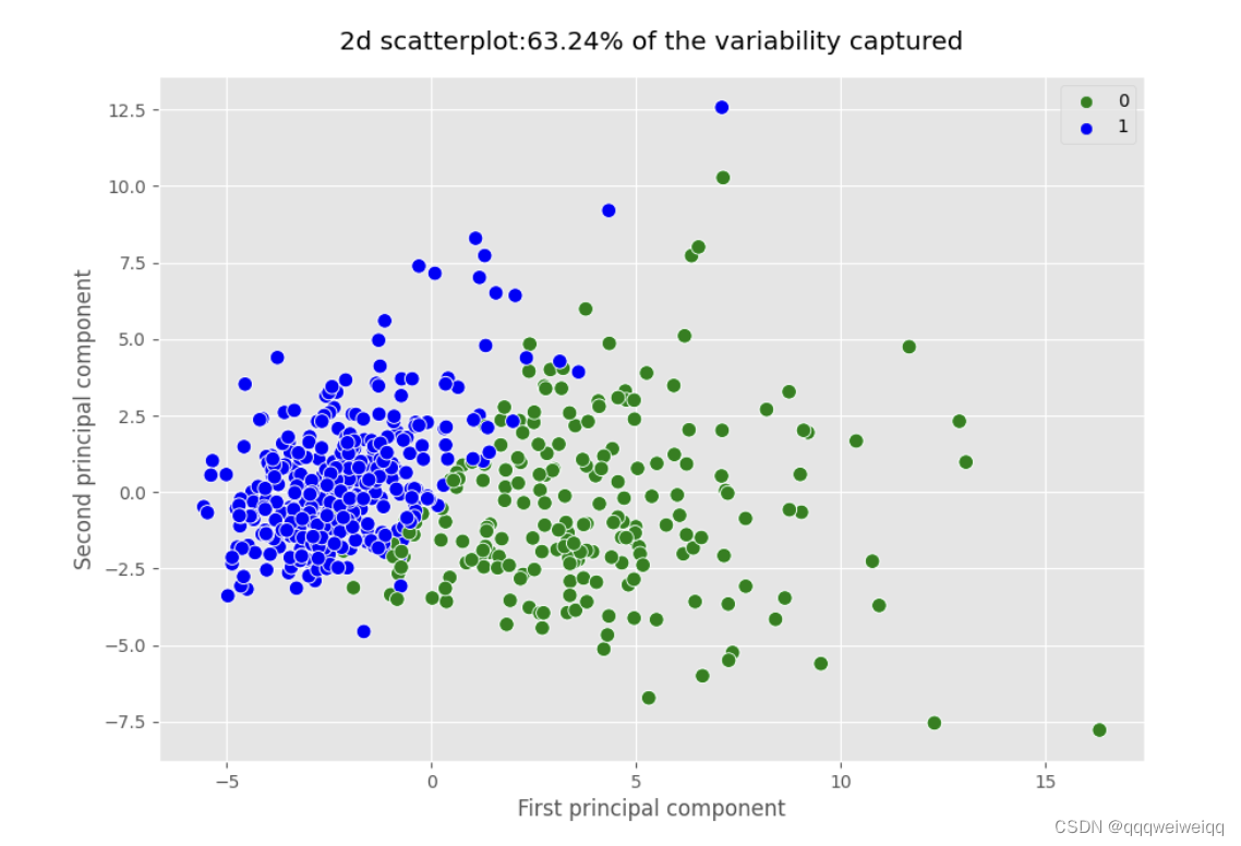
pca_2 = PCA(n_components=2,random_state=2020)
pca_2.fit(x_scaled)
x_pca_2=pca_2.transform(x_scaled)
plt.figure(figsize=(10,7))
sns.scatterplot(x=x_pca_2[:,0],y=x_pca_2[:,1],s=70,hue=cancer.target,palette=['green','blue'])
plt.title("2d scatterplot:63.24% of the variability captured",pad=15)
plt.xlabel("First principal component")
plt.ylabel("Second principal component")
plt.savefig('2d_scatterplot.png')



# ___________————————————————————————————————

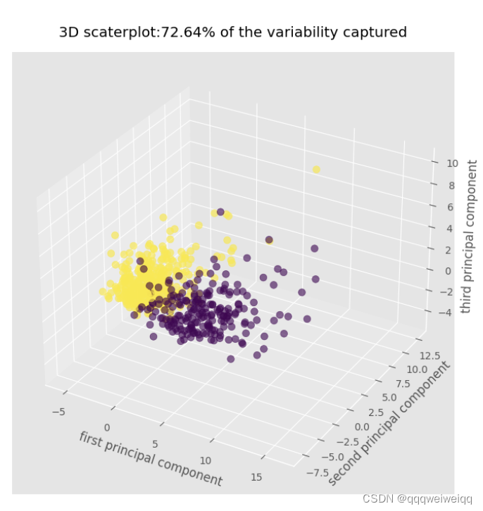
pca_3 = PCA(n_components=3,random_state=2020)
pca_3.fit(x_scaled)
x_pca_3=pca_3.transform(x_scaled)


fig= plt.figure(figsize=(12,8))

ax=plt.axes(projection='3d')

sctt=ax.scatter3D(x_pca_3[:,0],x_pca_3[:,1],x_pca_3[:,2],c=cancer.target,s=50,alpha=0.6)

plt.title("3D scaterplot:72.64% of the variability captured",pad=15)
ax.set_xlabel("first principal component")
ax.set_ylabel("second principal component")
ax.set_zlabel("third principal component")
plt.savefig('3d_scatterplot.png')