


LSTM简介
-
LSTM(Long Short-Term Memory)是一种特殊类型的循环神经网络(RNN),它在处理序列数据和时间序列数据时表现出色。
-
相比于传统的RNN,LSTM引入了记忆单元(memory cell)和门控机制(gate mechanism),以解决传统RNN中的梯度消失和梯度爆炸问题,从而更好地捕捉长期依赖关系。
-
LSTM的核心组件是记忆单元,它可以存储和访问信息,并通过门控机制来控制信息的流动。LSTM中的三种门控单元是:
 输入门(Input Gate):控制是否将新输入信息添加到记忆单元中。
 遗忘门(Forget Gate):控制记忆单元中的哪些信息需要被遗忘。
 输出门(Output Gate):控制从记忆单元中读取哪些信息并输出。
这些门通过使用sigmoid激活函数来产生0到1之间的输出,表示信息的通过程度。
- LSTM在训练过程中可以学习到如何选择存储和遗忘信息,从而对输入序列建模并捕捉到长期依赖关系。
- 除了标准的LSTM,还有一些变种模型,如双向LSTM(Bidirectional LSTM)、多层LSTM(Multi-layer LSTM)和注意力机制LSTM(LSTM with Attention),它们进一步扩展了LSTM的能力和灵活性。
数据集简介
北京PM2.5数据集
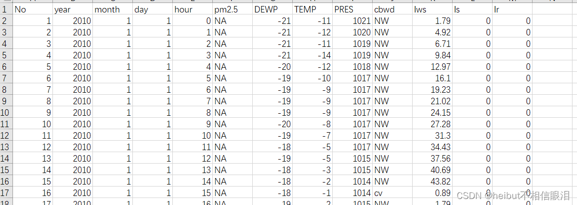
下载数据集并将其放在当前工作目录中,文件名为 “ raw.csv ”。
这是一个报告了中国北京美国大使馆五年每个小时的天气和污染程度的数据集。
- No:行号
- year:这一行中的数据年份
- month:此行中的数据月份
- day:这一行中的数据日
- hour:此行中的小时数据
- pm2.5:PM2.5浓度
- DEWP:露点
- TEMP:温度
- PRES:压力
- cbwd:综合风向
- Iws:累计风速
- Is:累积下了几个小时的雪
- Ir:累积下了几个小时的雨
我们可以使用这些数据,并构建一个预测问题,在前一时刻的天气条件和污染情况下,我们预测下一个时刻的污染情况。
数据预处理
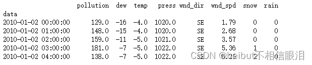
原始数据:
对原始数据处理:
from pandas import read_csv
from datetime import datetime
# 加载数据
def parse(x):
    return datetime.strptime(x,'%Y %m %d %H')
dataset=read_csv('data/raw.csv',parse_dates=[['year','month','day','hour']],index_col=0,date_parser=parse)
dataset.drop('No',axis=1,inplace=True)
# 手动更改列名
dataset.columns=['pollution','dew','temp','press','wnd_dir','wnd_spd','snow','rain']
dataset.index.name='data'
# 把所有NA值用0替换
dataset['pollution'].fillna(0,inplace=True)
dataset=dataset[24:]
# 输出前五行
print(dataset.head(5))
# 保存到文件中
dataset.to_csv('pollution.csv')
对以上代码进行解释:
- 将日期 - 时间信息合并成一个日期 - 时间,以便我们可以将它用作Pandas的一个索引。
- “No”列被删除,"inplace=True"时,表示对原始对象进行就地修改,而不是创建一个新的对象。
- 为每列指定更清晰的名称。最后,将NA值替换为“0”值,并且将前24小时移除。
- 运行该示例将输出转换数据集的前5行,并将数据集保存为“ pollution.csv ”。
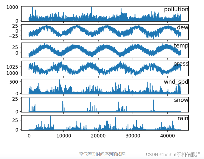
接下来查看我们的数据:
from pandas import read_csv
from matplotlib import pyplot
# 加载数据集
dataset=read_csv('data/pollution.csv',header=0,index_col=0)
values=dataset.values
# 指定要绘制的列
groups=[0,1,2,3,5,6,7]
i=1
# 绘制每一列
pyplot.figure()
for group in groups:
    pyplot.subplot(len(groups),1,i)
    pyplot.plot(values[:,group])
    pyplot.title(dataset.columns[group],y=0.5,loc='right')
    i+=1
pyplot.show()
多元LSTM预测模型
数据准备:
- 将数据集构造为监督学习问题并对输入变量进行归一化。
- 使用series_to_supervised()函数来转换数据集
# 将序列转换成监督学习问题
def series_to_supervised(data, n_in=1, n_out=1, dropnan=True):
n_vars = 1 if type(data) is list else data.shape[1]
df = DataFrame(data)
cols, names = list(), list()
# input sequence (t-n, ... t-1)
for i in range(n_in, 0, -1):
cols.append(df.shift(i))
names += [('var%d(t-%d)' % (j+1, i)) for j in range(n_vars)]
# forecast sequence (t, t+1, ... t+n)
for i in range(0, n_out):
cols.append(df.shift(-i))
if i == 0:
names += [('var%d(t)' % (j+1)) for j in range(n_vars)]
else:
names += [('var%d(t+%d)' % (j+1, i)) for j in range(n_vars)]
# put it all together
agg = concat(cols, axis=1)
agg.columns = names
# drop rows with NaN values
if dropnan:
agg.dropna(inplace=True)
return agg
# 加载数据集
dataset = read_csv('pollution.csv', header=0, index_col=0)
values = dataset.values
# 整数编码方向
encoder = LabelEncoder()
values[:,4] = encoder.fit_transform(values[:,4])
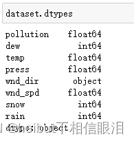
# 确保所有数据是浮动的
values = values.astype('float32')
# 归一化特征
scaler = MinMaxScaler(feature_range=(0, 1))
scaled = scaler.fit_transform(values)
# 构建成监督学习问题
reframed = series_to_supervised(scaled, 1, 1)
# 丢弃我们不想预测的列
reframed.drop(reframed.columns[[9,10,11,12,13,14,15]], axis=1, inplace=True)
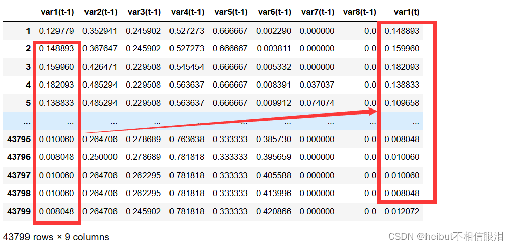
print(reframed.head())
结果展示:
   var1(t-1)  var2(t-1)  var3(t-1)  var4(t-1)  var5(t-1)  var6(t-1)  \
1   0.129779   0.352941   0.245902   0.527273   0.666667   0.002290
2   0.148893   0.367647   0.245902   0.527273   0.666667   0.003811
3   0.159960   0.426471   0.229508   0.545454   0.666667   0.005332
4   0.182093   0.485294   0.229508   0.563637   0.666667   0.008391
5   0.138833   0.485294   0.229508   0.563637   0.666667   0.009912

   var7(t-1)  var8(t-1)   var1(t)
1   0.000000        0.0  0.148893
2   0.000000        0.0  0.159960
3   0.000000        0.0  0.182093
4   0.037037        0.0  0.138833
5   0.074074        0.0  0.109658
对以上代码进行解释:
-
encoder = LabelEncoder() values[:,4] = encoder.fit_transform(values[:,4])对第四列wnd_dir列进行处理,将object类型转化成整数
-
series_to_supervised()函数中的shift(i)是将整列向上移动i个单位。
-
series_to_supervised()函数的作用:将第一列的数据向上以一格,存储到最后一列。
-
注意
n_in=1,n_out=1,用一个时间步长预测一个时间步长
定义和拟合模型
- 将第一年的数据作为训练集
- 前几列特征作为输入,最后一列为预测输出
from sklearn.preprocessing import LabelEncoder
from sklearn.preprocessing import MinMaxScaler
from pandas import DataFrame
from pandas import concat
# 把数据分为训练集和测试集
values = reframed.values
n_train_hours = 365 * 24
train = values[:n_train_hours, :]
test = values[n_train_hours:, :]
# 把数据分为输入和输出
train_X, train_y = train[:, :-1], train[:, -1]
test_X, test_y = test[:, :-1], test[:, -1]
# 把输入重塑成3D格式 [样例, 时间步, 特征]
train_X = train_X.reshape((train_X.shape[0], 1, train_X.shape[1]))
test_X = test_X.reshape((test_X.shape[0], 1, test_X.shape[1]))
print(train_X.shape, train_y.shape, test_X.shape, test_y.shape)
- 在第一隐层中定义50个神经元,在输出层中定义1个神经元用于预测污染。输入形状将是带有8个特征的一个时间步。
model.add(Dense(1))在神经网络模型中添加一个全连接层- 使用平均绝对误差(MAE)损失函数和随机梯度下降的高效Adam版本。
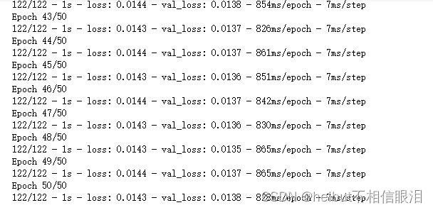
- 批量大小为72的50个训练时期
verbose=2, shuffle=False在每个epoch结束后输出一行记录。每个epoch训练数据将按照原始顺序进行训练
# 设计网络
model = Sequential()
model.add(LSTM(50, input_shape=(train_X.shape[1], train_X.shape[2])))
model.add(Dense(1))
model.compile(loss='mae', optimizer='adam')
# 拟合网络
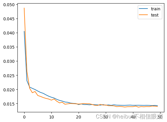
history = model.fit(train_X, train_y, epochs=50, batch_size=72, validation_data=(test_X, test_y), verbose=2, shuffle=False)
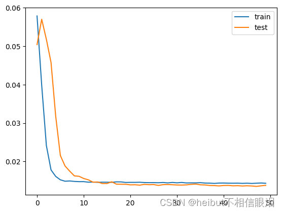
# 绘制历史数据
pyplot.plot(history.history['loss'], label='train')
pyplot.plot(history.history['val_loss'], label='test')
pyplot.legend()
pyplot.show()
评估模型
from keras.models import Sequential
from keras.layers import LSTM, Dense
from sklearn.metrics import mean_squared_error
# 做出预测
yhat = model.predict(test_X)
test_X = test_X.reshape((test_X.shape[0], test_X.shape[2]))
# 反向转换预测值比例
inv_yhat = np.concatenate((yhat, test_X[:, 1:]), axis=1)
inv_yhat = scaler.inverse_transform(inv_yhat)
inv_yhat = inv_yhat[:,0]
# 反向转换实际值比例
test_y = test_y.reshape((len(test_y), 1))
inv_y = np.concatenate((test_y, test_X[:, 1:]), axis=1)
inv_y = scaler.inverse_transform(inv_y)
inv_y = inv_y[:,0]
# 计算RMSE
rmse = np.sqrt(mean_squared_error(inv_y, inv_yhat))
print('Test RMSE: %.3f' % rmse)
1095/1095 [==============================] - 1s 1ms/step
Test RMSE: 26.628
训练多个滞后时间步
用多个时间步长去预测一个时间步长,将n_in=1,传入参数改为n_in=n_hours=3,n_features=8。
反向转换预测值比例 inv_yhat = concatenate((yhat, test_X
[:, -7:]), axis=1)
inv_yhat = scaler.inverse_transform(inv_yhat) inv_yhat = inv_yhat[:,0]
反向转换实际值大小 test_y = test_y.reshape((len(test_y), 1)) inv_y =
concatenate((test_y, test_X[:, -7:]), axis=1) inv_y =
scaler.inverse_transform(inv_y) inv_y = inv_y[:,0]
为什么 concatenate((test_y, test_X[:, -7:]), axis=1)里面的test_X可以选择任意的七列???在线求解
from math import sqrt
from numpy import concatenate
from matplotlib import pyplot
from pandas import read_csv
from pandas import DataFrame
from pandas import concat
from sklearn.preprocessing import MinMaxScaler
from sklearn.preprocessing import LabelEncoder
from sklearn.metrics import mean_squared_error
from keras.models import Sequential
from keras.layers import Dense
from keras.layers import LSTM
# 将序列转换为监督学习问题
def series_to_supervised(data, n_in=1, n_out=1, dropnan=True):
    n_vars = 1 if type(data) is list else data.shape[1]
    df = DataFrame(data)
    cols, names = list(), list()
    # input sequence (t-n, ... t-1)
    for i in range(n_in, 0, -1):
        cols.append(df.shift(i))
        names += [('var%d(t-%d)' % (j+1, i)) for j in range(n_vars)]
    # forecast sequence (t, t+1, ... t+n)
    for i in range(0, n_out):
        cols.append(df.shift(-i))
        if i == 0:
            names += [('var%d(t)' % (j+1)) for j in range(n_vars)]
        else:
            names += [('var%d(t+%d)' % (j+1, i)) for j in range(n_vars)]
    # put it all togethe
    agg = concat(cols, axis=1)
    agg.columns = names
    # drop rows with NaN values
    if dropnan:
        agg.dropna(inplace=True)
    return agg
# 加载数据集
dataset = read_csv('data/pollution.csv', header=0, index_col=0)
values = dataset.values
# 整数编码
encoder = LabelEncoder()
values[:,4] = encoder.fit_transform(values[:,4])
# 确保所有数据是浮动的
values = values.astype('float32')
# 归一化特征
scaler = MinMaxScaler(feature_range=(0, 1))
scaled = scaler.fit_transform(values)
# 指定滞后时间大小
n_hours = 3
n_features = 8
# 构建监督学习问题
reframed = series_to_supervised(scaled, n_hours, 1)
#将除了PM2.5的其余列丢弃
reframed.drop(reframed.columns[[25,26,27,28,29,30,31]], axis=1, inplace=True)
print(reframed.shape)
(43797, 25)
var1(t-3)	var2(t-3)	var3(t-3)	var4(t-3)	var5(t-3)	var6(t-3)	var7(t-3)	var8(t-3)	var1(t-2)	var2(t-2)	...	var8(t-2)	var1(t-1)	var2(t-1)	var3(t-1)	var4(t-1)	var5(t-1)	var6(t-1)	var7(t-1)	var8(t-1)	var1(t)
3	0.129779	0.352941	0.245902	0.527273	0.666667	0.002290	0.000000	0.0	0.148893	0.367647	...	0.0	0.159960	0.426471	0.229508	0.545454	0.666667	0.005332	0.000000	0.0	0.182093
4	0.148893	0.367647	0.245902	0.527273	0.666667	0.003811	0.000000	0.0	0.159960	0.426471	...	0.0	0.182093	0.485294	0.229508	0.563637	0.666667	0.008391	0.037037	0.0	0.138833
5	0.159960	0.426471	0.229508	0.545454	0.666667	0.005332	0.000000	0.0	0.182093	0.485294	...	0.0	0.138833	0.485294	0.229508	0.563637	0.666667	0.009912	0.074074	0.0	0.109658
6	0.182093	0.485294	0.229508	0.563637	0.666667	0.008391	0.037037	0.0	0.138833	0.485294	...	0.0	0.109658	0.485294	0.213115	0.563637	0.666667	0.011433	0.111111	0.0	0.105634
7	0.138833	0.485294	0.229508	0.563637	0.666667	0.009912	0.074074	0.0	0.109658	0.485294	...	0.0	0.105634	0.485294	0.213115	0.581818	0.666667	0.014492	0.148148	0.0	0.124748
...	...	...	...	...	...	...	...	...	...	...	...	...	...	...	...	...	...	...	...	...	...
43795	0.008048	0.250000	0.311475	0.745455	0.333333	0.365103	0.000000	0.0	0.009054	0.264706	...	0.0	0.010060	0.264706	0.278689	0.763638	0.333333	0.385730	0.000000	0.0	0.008048
43796	0.009054	0.264706	0.295082	0.763638	0.333333	0.377322	0.000000	0.0	0.010060	0.264706	...	0.0	0.008048	0.250000	0.278689	0.781818	0.333333	0.395659	0.000000	0.0	0.010060
43797	0.010060	0.264706	0.278689	0.763638	0.333333	0.385730	0.000000	0.0	0.008048	0.250000	...	0.0	0.010060	0.264706	0.262295	0.781818	0.333333	0.405588	0.000000	0.0	0.010060
43798	0.008048	0.250000	0.278689	0.781818	0.333333	0.395659	0.000000	0.0	0.010060	0.264706	...	0.0	0.010060	0.264706	0.262295	0.781818	0.333333	0.413996	0.000000	0.0	0.008048
43799	0.010060	0.264706	0.262295	0.781818	0.333333	0.405588	0.000000	0.0	0.010060	0.264706	...	0.0	0.008048	0.264706	0.245902	0.781818	0.333333	0.420866	0.000000	0.0	0.012072
43797 rows × 25 columns
# 分为训练集和测试集
values = reframed.values
n_train_hours = 365 * 24
train = values[:n_train_hours, :]
test = values[n_train_hours:, :]
# 分为输入和输出
n_obs = n_hours * n_features
train_X, train_y = train[:, :-1], train[:, -1]
test_X, test_y = test[:, :-1], test[:, -1]
print(train_X.shape, len(train_X), train_y.shape)
# 重塑为3D形状 [samples, timesteps, features]
n_features = 8
train_X = train_X.reshape((train_X.shape[0], n_hours, n_features))
test_X = test_X.reshape((test_X.shape[0], n_hours, n_features))
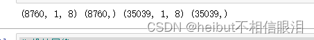
print(train_X.shape, train_y.shape, test_X.shape, test_y.shape)
(8760, 24) 8760 (8760,)
(8760, 3, 8) (8760,) (35037, 3, 8) (35037,)
模型中的最后一层是一个具有1个神经元的全连接层(Dense),因此预测结果将是train_y.shape[1]列。

# 设计网络
model = Sequential()
model.add(LSTM(50, input_shape=(train_X.shape[1], train_X.shape[2])))
model.add(Dense(1))
model.compile(loss='mae', optimizer='adam')
# 拟合网络模型
history = model.fit(train_X, train_y, epochs=50, batch_size=72, validation_data=(test_X, test_y), verbose=2, shuffle=False)
# 绘制历史数据
pyplot.plot(history.history['loss'], label='train')
pyplot.plot(history.history['val_loss'], label='test')
pyplot.legend()
pyplot.show()
# 作出预测
yhat = model.predict(test_X)
test_X = test_X.reshape((test_X.shape[0], n_hours*n_features))
# 反向转换预测值比例
inv_yhat = concatenate((yhat, test_X[:, :7]), axis=1)
inv_yhat = scaler.inverse_transform(inv_yhat)
inv_yhat = inv_yhat[:,0]
# 反向转换实际值大小
test_y = test_y.reshape((len(test_y), 1))
inv_y = concatenate((test_y, test_X[:, :7]), axis=1)
inv_y = scaler.inverse_transform(inv_y)
inv_y = inv_y[:,0]
# 计算RMSE大小
rmse = sqrt(mean_squared_error(inv_y, inv_yhat))
print('Test RMSE: %.3f' % rmse)
1095/1095 [==============================] - 2s 1ms/step
Test RMSE: 26.396
26.396与26.628相比没有差很多,并没有真正显示出技术上的优势。


 3547
3547


 被折叠的 条评论
为什么被折叠?
被折叠的 条评论
为什么被折叠?
 到【灌水乐园】发言


