吴恩达机器学习-异常检测（Anomaly Detection）

在本练习中，您将实现异常检测算法，并将其应用于检测网络上出现故障的服务器。

1-包

首先，让我们运行下面的单元格来导入此分配过程中需要的所有包。
numpy是在Python中处理矩阵的基本包。
matplotlib是一个著名的Python绘图库。
utils.py包含此赋值的辅助函数。您不需要修改此文件中的代码。

import numpy as np
import matplotlib.pyplot as plt
from utils import *

%matplotlib inline

2-异常检测

2.1问题陈述

在本练习中，您将实现一种异常检测算法来检测服务器计算机中的异常行为。
数据集包含两个特征-

• 每个服务器的响应吞吐量（mb/s）和延迟（ms）。

当您的服务器运行时，您收集了𝑚=307他们的行为示例，因此有一个未标记的数据集{𝑥(1)…𝑥(𝑚)}

• 您怀疑这些例子中的绝大多数都是服务器正常运行的“正常”（非异常）例子，但也可能有一些服务器在该数据集中表现异常的例子。

您将使用高斯模型来检测数据集中的异常示例。

• 您将首先从2D数据集开始，该数据集将允许您可视化算法正在做的事情。
• 在该数据集上，您将拟合高斯分布，然后找到概率非常低的值，因此可以被视为异常。
• 之后，您将把异常检测算法应用于具有多个维度的更大数据集。

2.2数据集

您将从加载此任务的数据集开始。
下面显示的load_data（）函数将数据加载到变量X_train、X_val和y_val中。您将使用X_train来拟合高斯分布。您将用X_val和y_val作为交叉验证集来选择阈值并确定异常与正常示例

# Load the dataset
X_train, X_val, y_val = load_data()

查看变量
让我们更熟悉您的数据集。
一个好的开始是打印出每个变量，看看它包含什么。
下面的代码打印每个变量的前五个元素

# Display the first five elements of X_train
print("The first 5 elements of X_train are:\n", X_train[:5])  

The first 5 elements of X_train are:
 [[13.04681517 14.74115241]
 [13.40852019 13.7632696 ]
 [14.19591481 15.85318113]
 [14.91470077 16.17425987]
 [13.57669961 14.04284944]]

# Display the first five elements of X_val
print("The first 5 elements of X_val are\n", X_val[:5])  

The first 5 elements of X_val are
 [[15.79025979 14.9210243 ]
 [13.63961877 15.32995521]
 [14.86589943 16.47386514]
 [13.58467605 13.98930611]
 [13.46404167 15.63533011]]

# Display the first five elements of y_val
print("The first 5 elements of y_val are\n", y_val[:5])  

The first 5 elements of y_val are
 [0 0 0 0 0]

👆这个输出代表的是前五个数据是没有异常

检查变量的维度
熟悉数据的另一种有用方法是查看其维度。
下面的代码打印X_train、X_val和y_val的形状。

print ('The shape of X_train is:', X_train.shape)
print ('The shape of X_val is:', X_val.shape)
print ('The shape of y_val is: ', y_val.shape)

The shape of X_train is: (307, 2)
The shape of X_val is: (307, 2)
The shape of y_val is:  (307,)

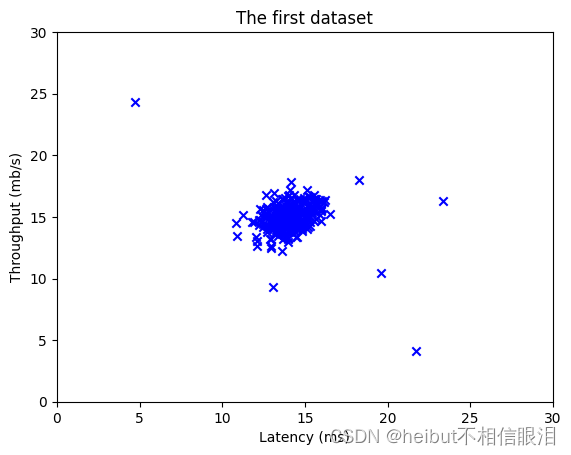
可视化数据
在开始执行任何任务之前，通过可视化数据来理解数据通常是很有用的。

• 对于这个数据集，您可以使用散点图来可视化数据（X_train），因为它只有两个属性要绘制（吞吐量和延迟）
• 你的情节应该与下面的相似

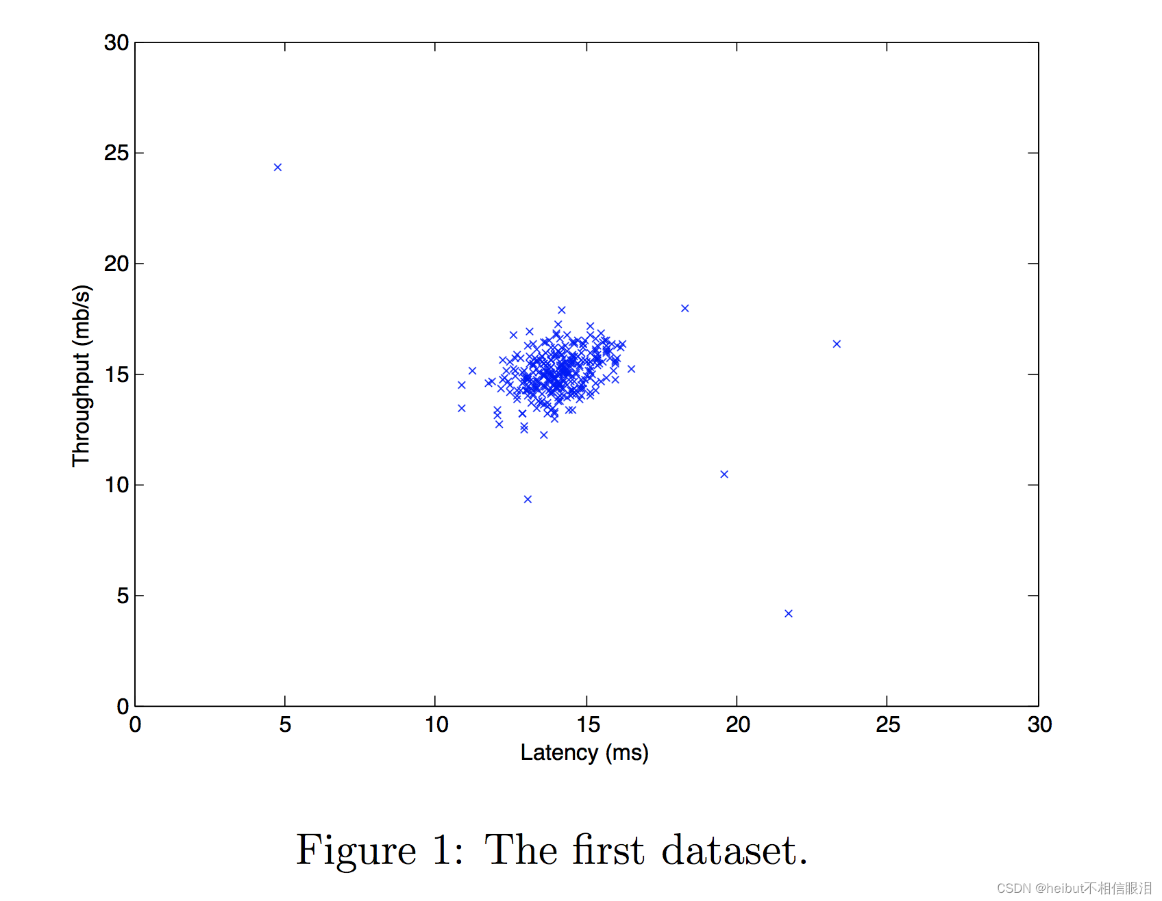
# Create a scatter plot of the data. To change the markers to blue "x",
# we used the 'marker' and 'c' parameters
plt.scatter(X_train[:, 0], X_train[:, 1], marker='x', c='b') 

# Set the title
plt.title("The first dataset")
# Set the y-axis label
plt.ylabel('Throughput (mb/s)')
# Set the x-axis label
plt.xlabel('Latency (ms)')
# Set axis range
plt.axis([0, 30, 0, 30])
plt.show()

2.3高斯分布

要进行异常检测，首先需要根据数据的分布拟合模型。

• 提供一套训练集{𝑥1…𝑥(𝑚)}要估计每个特征𝑥𝑖的高斯分布
• 回想一下，高斯分布
  
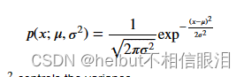
  𝜇是均值和𝜎2控制方差。
• 这段话是在描述一个参数估计的问题，其中有 𝑛 个特征（或者说维度），每个特征有一组数据
  {𝑥(1)𝑖,…,𝑥(𝑚)𝑖}，其中 𝑚 是样本数量。问题的目标是为每个特征找到合适的参数 𝜇𝑖 和
  𝜎2𝑖，这些参数可以用来描述这些数据的分布情况。

具体来说，𝜇𝑖 是数据在第 𝑖 维的均值（平均值），而 𝜎2𝑖 则是数据在第 𝑖
维的方差（或标准差的平方）。通过估计这些参数，我们可以更好地了解数据在每个维度上的分布特征，从而进行进一步的分析或建模。

2.2.1高斯实现的估计参数：

您的任务是完成下面estimate_gaussian中的代码。

练习1
请完成下面的estimate_gaussian函数，以计算μ（X中每个特征的平均值）和var（X中各个特征的方差）。
您可以估计参数（𝜇𝑖, 𝜎𝑖^2)。要估计平均值，您将使用：
如果遇到问题，可以查看下面单元格后面的提示，以帮助您实现。

# UNQ_C1
# GRADED FUNCTION: estimate_gaussian

def estimate_gaussian(X): 
    """
    Calculates mean and variance of all features 
    in the dataset
    
    Args:
        X (ndarray): (m, n) Data matrix
    
    Returns:
        mu (ndarray): (n,) Mean of all features
        var (ndarray): (n,) Variance of all features
    """

    m, n = X.shape
 
    mu = np.mean(X, axis=1)
    var = np.var(X, axis=1)
    ### START CODE HERE ### 
    mu=1/m *np.sum(X,axis=0)
    var=1/m *np.sum((X-mu)**2,axis=0)
    ### END CODE HERE ### 
        
    return mu, var

您可以通过运行以下测试代码来检查您的实现是否正确：

# Estimate mean and variance of each feature
mu, var = estimate_gaussian(X_train)              

print("Mean of each feature:", mu)
print("Variance of each feature:", var)
    
# UNIT TEST
from public_tests import *
estimate_gaussian_test(estimate_gaussian)

Mean of each feature: [14.11222578 14.99771051]
Variance of each feature: [1.83263141 1.70974533]
All tests passed!

Expected Output:

Mean of each feature:	[14.11222578 14.99771051]
Variance of each feature:	[1.83263141 1.70974533]

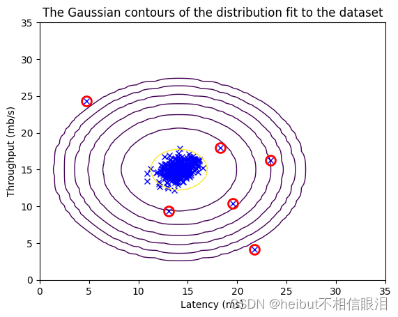
现在您已经完成了estimate_gaussian中的代码，我们将可视化拟合的高斯分布的轮廓。
你应该得到一个类似下图的图。

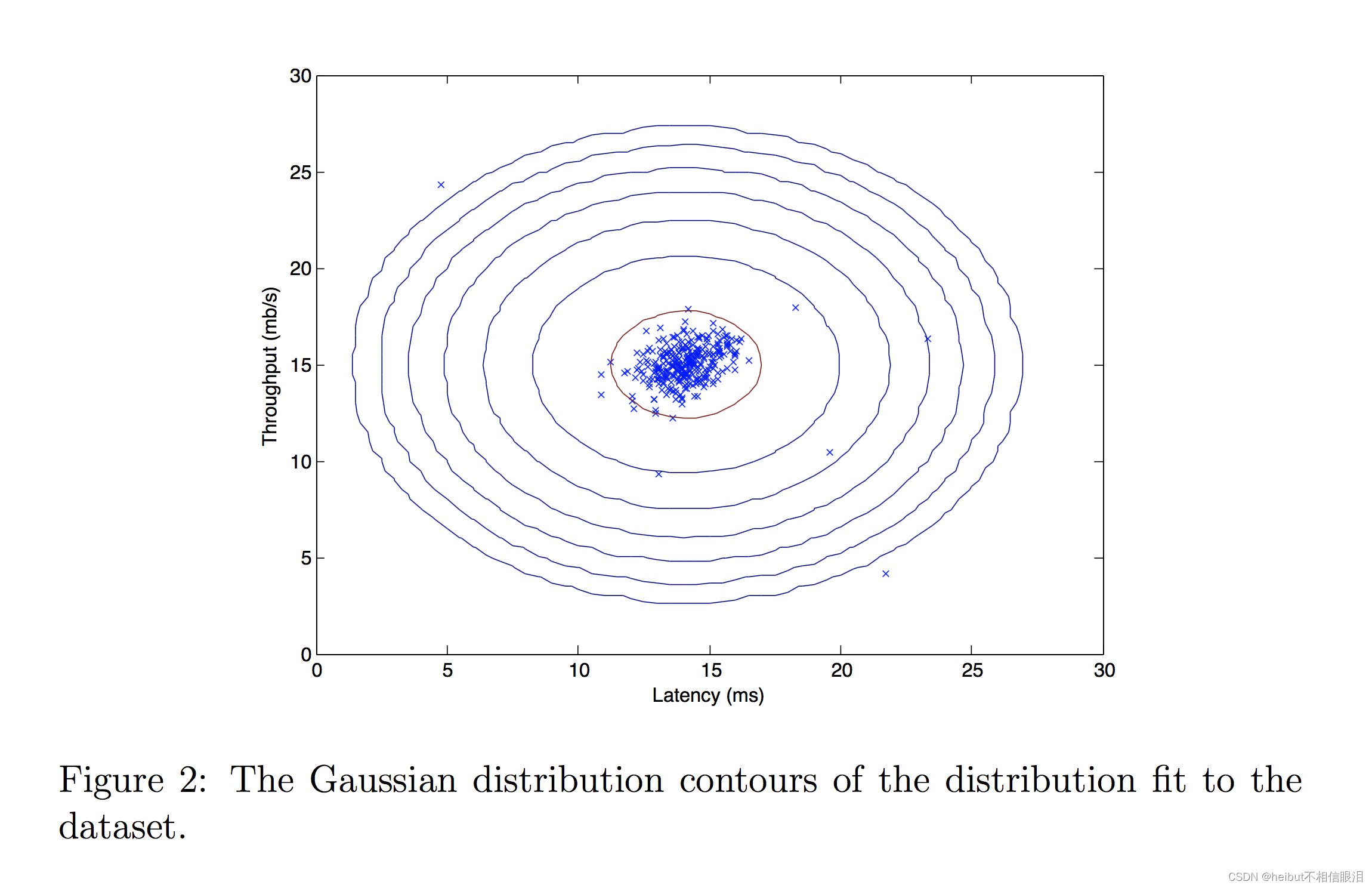
从你的图表中，你可以看到大多数例子都在概率最高的地区，而异常例子则在概率较低的地区。

# Returns the density of the multivariate normal
# at each data point (row) of X_train
p = multivariate_gaussian(X_train, mu, var)

#Plotting code 
visualize_fit(X_train, mu, var)

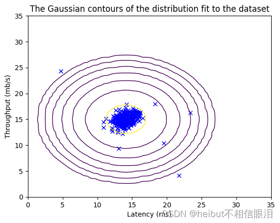
这段代码涉及多元高斯分布的概率密度函数以及可视化其拟合结果。

1. multivariate_gaussian(X_train, mu, var): 这个函数计算多元高斯分布在训练数据集 X_train 中每个数据点处的概率密度值。参数 mu 是多元高斯分布的均值向量，var 是协方差矩阵。

2. visualize_fit(X_train, mu, var): 这个函数用于可视化多元高斯分布拟合的结果。它可能会在训练数据集 X_train
   的散点图上叠加绘制等高线或者三维曲面，以展示多元高斯分布在数据空间中的拟合情况。这样可以直观地观察模型对数据的拟合程度以及数据的分布情况。

2.2.2选择阈值𝜖

既然你已经估计了高斯参数，你就可以研究在给定这种分布的情况下，哪些例子的概率非常高，而哪些例子的可能性非常低。

• 低概率的例子更有可能是我们数据集中的异常。
• 确定哪些示例是异常的一种方法是基于交叉验证集选择阈值。

在本节中，您将完成select_threshold中的代码使用𝐹1在交叉验证集上得分，以选择阈值𝜀

𝑚 是样本数量

• 为此，我们将使用交叉验证集{(𝑥cv^(1)，𝑦 cv^(1)),......,(𝑥 cv^(𝑚cv)，𝑦cv^(𝑚cv))}，其中标签𝑦=1.对应于异常示例，并且𝑦=0,对应于正常示例。
• 对于每个交叉验证示例，我们将计算𝑝(𝑥cv^(𝑖)）.所有这些概率的矢量𝑝(𝑥cv^(1)），…，𝑝(𝑥(𝑚cv)）被传递到向量p_val中的select_threshold。
• 相应的标签𝑦cv^(1)，…，𝑦cv^(𝑚cv）被传递给向量y_ val中的相同函数。

对上述说明进行解释：

假设我们有一个交叉验证集，其中包含三个样本，每个样本有两个特征。这个交叉验证集可以表示为一组元组，每个元组包含一个特征向量和一个标签。假设这些样本如下：

样本1：特征向量为 [5.1, 3.5]，标签为 0（表示正常样本） 样本2：特征向量为 [4.9, 3.0]，标签为 1（表示异常样本）
样本3：特征向量为 [6.0, 2.7]，标签为 0（表示正常样本） 则这个交叉验证集可以表示为如下形式的元组：

[([5.1, 3.5], 0), ([4.9, 3.0], 1), ([6.0, 2.7], 0)]

对于交叉验证集中的每个样本，计算其在训练好的多元高斯模型下的概率密度值，即 𝑝(𝑥(𝑖)cv)。

将所有样本的概率密度值组成向量，记为 p_val。

同时，将交叉验证集中的所有样本的真实标签组成向量，记为 y_val。

将概率密度向量 p_val 和真实标签向量 y_val 传递给select_threshold，该函数用于根据概率密度和真实标签选择一个合适的阈值，以区分正常样本和异常样本。这个阈值可以用于根据模型输出的概率密度值判断一个样本是否为异常

练习2
请完成下面的select_threshold函数，根据验证集（p_val）和基本事实（y_val）的结果，找到用于选择异常值的最佳阈值。

• 在提供的代码select_threshold中，已经有一个循环将尝试的许多不同值𝜀，并基于𝐹1分数选择最好的𝜀

• 您需要实现代码，通过选择epsilon作为阈值来计算F1分数，并将值放在F1中。

  • 回想一下，如果一个例子𝑥概率很低𝑝(𝑥)<𝜀，则将其归类为异常。

  • 然后，您可以通过以下方式计算精度和召回率：

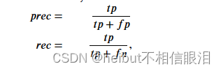
  • 𝑡𝑝是真阳性的数量：地面实况标签说这是一个异常，我们的算法正确地将其归类为异常。

  • 𝑓𝑝是误报的数量：基本事实标签说这不是异常，但我们的算法错误地将其归类为异常。

  • 𝑓𝑛是假阴性的数量：地面实况标签说这是异常，但我们的算法错误地将其归类为非异常。

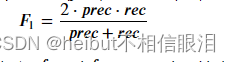
• 这个𝐹1.使用精度（𝑝𝑟𝑒𝑐)和召回（𝑟𝑒𝑐)如下所示：

**实施说明：**为了计算𝑡𝑝, 𝑓𝑝和𝑓𝑛，您可能能够使用矢量化实现，而不是在所有示例上循环。
如果遇到问题，可以查看下面单元格后面的提示，以帮助您实现。

def select_threshold(y_val, p_val): 
    """
    Finds the best threshold to use for selecting outliers 
    based on the results from a validation set (p_val) 
    and the ground truth (y_val)
    
    Args:
        y_val (ndarray): Ground truth on validation set
        p_val (ndarray): Results on validation set
        
    Returns:
        epsilon (float): Threshold chosen 
        F1 (float):      F1 score by choosing epsilon as threshold
    """ 

    best_epsilon = 0
    best_F1 = 0
    F1 = 0
    
    step_size = (max(p_val) - min(p_val)) / 1000
    
    for epsilon in np.arange(min(p_val), max(p_val), step_size):
        # Predictions based on epsilon
        preds = (p_val < epsilon).astype(int)
        
        # True positives
        TP = np.sum((preds == 1) & (y_val == 1))
        
        # False positives
        FP = np.sum((preds == 1) & (y_val == 0))
        
        # False negatives
        FN = np.sum((preds == 0) & (y_val == 1))
        
        # Calculate precision and recall
        prec = TP / (TP + FP) if (TP + FP) != 0 else 0
        rec = TP / (TP + FN) if (TP + FN) != 0 else 0
        
        # Calculate F1 score
        F1 = (2 * prec * rec) / (prec + rec) if (prec + rec) != 0 else 0
        
        if F1 > best_F1:
            best_F1 = F1
            best_epsilon = epsilon
        
    return best_epsilon, best_F1

您可以使用以下代码检查您的实现

p_val = multivariate_gaussian(X_val, mu, var)
epsilon, F1 = select_threshold(y_val, p_val)

print('Best epsilon found using cross-validation: %e' % epsilon)
print('Best F1 on Cross Validation Set: %f' % F1)
    
# UNIT TEST
select_threshold_test(select_threshold)

Best epsilon found using cross-validation: 8.990853e-05
Best F1 on Cross Validation Set: 0.875000
All tests passed!

Expected Output:

Best epsilon found using cross-validation:	8.99e-05
Best F1 on Cross Validation Set:	0.875

现在，我们将运行您的异常检测代码，并在图中圈出异常（下图3）。

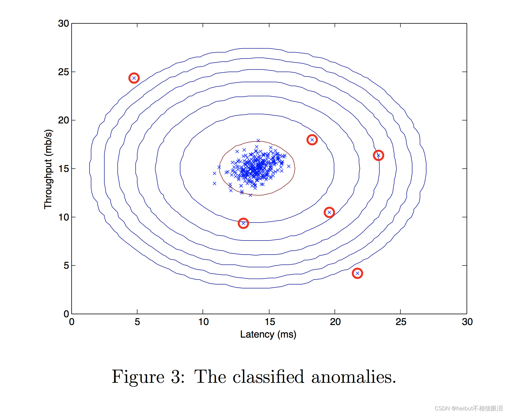
# Find the outliers in the training set 
outliers = p < epsilon

# Visualize the fit
visualize_fit(X_train, mu, var)

# Draw a red circle around those outliers
plt.plot(X_train[outliers, 0], X_train[outliers, 1], 'ro',
         markersize= 10,markerfacecolor='none', markeredgewidth=2)

2.4高维数据集

现在，我们将在更现实、更困难的数据集上运行您实现的异常检测算法。
在这个数据集中，每个示例都由11个特性描述，捕获了计算服务器的更多属性。
让我们从加载数据集开始。

• 下面显示的load_data（）函数将数据加载到变量X_train_high、X_val_high和y_val_high中
• _high是指将这些变量与前一部分中使用的变量区分开来。
• 我们将使用X_train_high来拟合高斯分布。
• 我们将用X_val_high和y_val_high作为交叉验证集来选择阈值并确定异常与正态示例

# load the dataset
X_train_high, X_val_high, y_val_high = load_data_multi()

检查变量的尺寸
让我们检查这些新变量的尺寸，以熟悉数据

print ('The shape of X_train_high is:', X_train_high.shape)
print ('The shape of X_val_high is:', X_val_high.shape)
print ('The shape of y_val_high is: ', y_val_high.shape)

The shape of X_train_high is: (1000, 11)
The shape of X_val_high is: (100, 11)
The shape of y_val_high is:  (100,)

异常检测
现在，让我们在这个新的数据集上运行异常检测算法。
下面的代码将使用您的代码

• 估计高斯参数（𝜇𝑖和𝜎i2)
• 评估用于估计高斯参数的训练数据X_train_high以及交叉验证集X_val_high的概率。
• 最后，它将使用select_threshold来找到最佳阈值𝜀 .

# Apply the same steps to the larger dataset

# Estimate the Gaussian parameters
mu_high, var_high = estimate_gaussian(X_train_high)

# Evaluate the probabilites for the training set
p_high = multivariate_gaussian(X_train_high, mu_high, var_high)

# Evaluate the probabilites for the cross validation set
p_val_high = multivariate_gaussian(X_val_high, mu_high, var_high)

# Find the best threshold
epsilon_high, F1_high = select_threshold(y_val_high, p_val_high)

print('Best epsilon found using cross-validation: %e'% epsilon_high)
print('Best F1 on Cross Validation Set:  %f'% F1_high)
print('# Anomalies found: %d'% sum(p_high < epsilon_high))

Best epsilon found using cross-validation: 1.377229e-18
Best F1 on Cross Validation Set:  0.615385
# Anomalies found: 117

Expected Output:

Best epsilon found using cross-validation:	1.38e-18
Best F1 on Cross Validation Set:	0.615385
# anomalies found:	117