Course2-week2-optimization algorithm

optimization algorithms

1 - mini-batch gradient descent

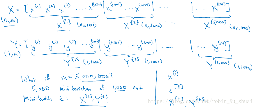
vectorization allows you to efficiently compute on m examples.But if m is large then it can be very slow. With the implement of graident descent on the whole training set, what we have to do that we process entire training set before we take one little step of gradient descent.And we have to process the entire training set before we take another step of gradient descent.

What we can do is split the giant training set into many baby subset, called mini-batch.

if m = 5,000,000,

$$X^{\{1\}} = (x^{(1)},x^{(2)},\cdots, x^{(1000)}), \cdots, X^{\{5000\}} = (x^{(4999000)},x^{(4999001)},\cdots, x^{(5000,000)})$$
similiarly do the same thing for $Y$, also split up the training data for $Y$ accordingly.

so mini-batch t is comprised of $X^{\{t\}}$ and $Y^{\{t\}}$.

Note:

• $x^{(i)}$ is the i^{th} training example
• $z^{[l]}$ refer to the $z$ value of the layer $l$
• $X^{\{t\}}$ and $Y^{\{t\}}$ denote the $t^{th}$ mini-batch

Let’s see how mini-batch gradient descent work?

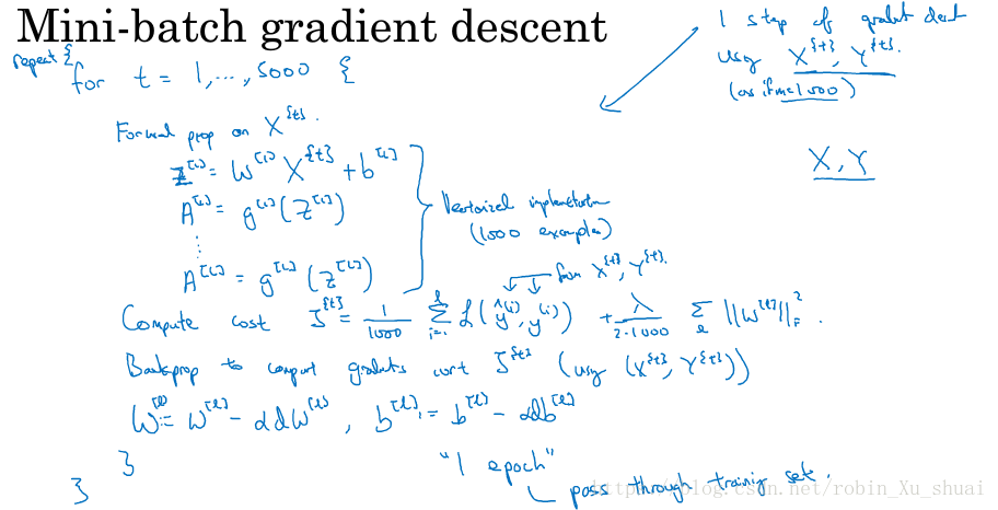
The code here is also called doing one Epoch of training set, Epoch is a word that means a single pass through the training set. So with the batch gradient descent, a Epoch allow you take only one gradient descent step, with mini-batch gradient descent, a single pass through the training set, that is one Epoch, allow you to take 5000 gradient descent steps.

When we have a lot training set, mini-batch run much faster than batch gradient descent.

2 - understanding mini-batch gradient descent

We will learn the detail how to implement the mini-bathc gradient descent and gain a better understanding of what it’s doing and why is work.

One of the size of parameters we need to choose is the size of mini-batch. let’s set m is the training set size.

• On one extreme, if the mini-batch is m, then we just end up with batch gradient descent.
• The another extreme would be if set mini-batch equals to 1, called stochastic gradient descent, here every examples is its own mini-batch, and looking just one training example to do one step of gradient descent.

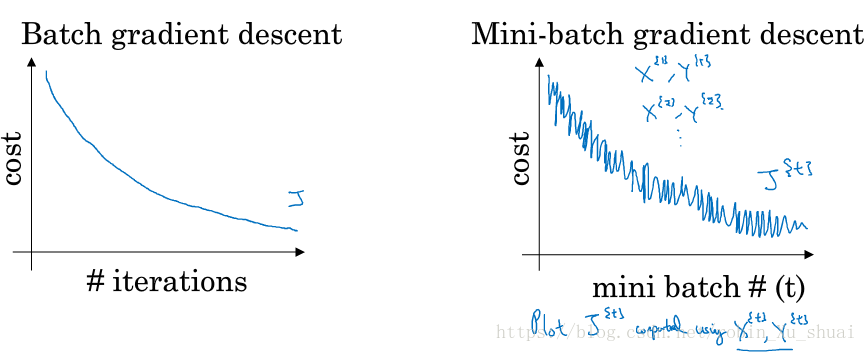
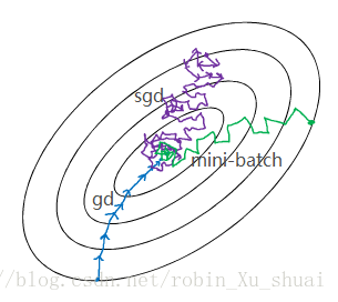
Stochastic gradient descent won’t ever converge. it’ll always just kind of oscillate and wander around the region of the minimum.

If using batch gradient descent, we are processing a huge training set on every iteration, the main disadvantage of this is that it takes too much time too long per iteration before take one step of gradient descent.

If we go to the opposite, using the stochastic gradient descent, the huge disadvantage is we will loss the speed up from vectorization. since we are processing a single training example at a time.

So work best in practice is somethings in between, when we have some mini-batch size not too big or too small, this will give us the faster learning. The advantage is:

• speed up from vectorization.
• without needing to wait till scan entire training set. On each epoch allows us to run many times gradient descent steps.

how do choose the mini-bathc size?

• if we have a small training set, just use batch gradient descent.
  
  • less than 2000
• if we have a large training set
  
  • mini-batch: 64, 128, 256, 215

3 - expononentially weighted average

We will talk about a few optimization algorithms, they are faster than gradient descent.

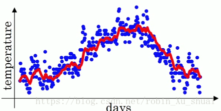
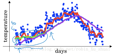
If we want to compute the trend, the local average or a moveing average of the temperatures span last year, $\theta_1 = 40F, \theta_2 = 49F, \cdots, \theta_{180} = 56F, \cdots$ Here is what we can do:

$$\begin{aligned} & V_0 = 0 \\ & V_1 = 0.9V_0 + 0.1\theta_1 \\ & V_2 = 0.9V_1 + 0.1\theta_2 \\ & \cdots\\ & V_t = 0.9V_{t-1} + 0.1\theta_t \\ \end{aligned}$$

In this way, we can get a exponentially weighted averages of the daily temperature show in the red line.

$$V_t = \beta V_{t-1} + (1-\beta)\theta_t$$

And when we compute this we can think of $V_t$ as approximately average over $\frac{1}{1 - \beta}$ daily temperature.

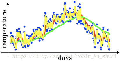
• $\beta = 0.9:$, averaging over rougly 10 daily temperature
• $\beta = 0.98:$, averaging over rougly 50 daily temperature, green line, adapts slowly to temperature changes
• $\beta = 0.5:$, averaging over rougly 2 daily temperature, yellow line, adapts quickly to temperature changes

4 - understanding exponentially weighted average

We talked about exponentially weighted average, this will turn out to be a key compontent of several optimization algorithms.
Here is the key euqation for implementing the exponentially weighted average,

$$V_t = \beta V_{t-1} + (1-\beta)\theta_t$$

Let’s look a bit more than that to understand how this is computing averages of the daily temperature.

$$\begin{aligned} & v_{100} = 0.9v_{99} + 0.1\theta_{100} \\ & v_{99} = 0.9v_{98} + 0.1\theta_{99} \\ & v_{98} = 0.9v_{97} + 0.1\theta_{98} \\ & \cdots \\ \end{aligned}$$

$$v_{100} = 0.1\theta_{100} + 0.9(0.1\theta_{99} + 0.9(0.1\theta_{98} + 0.9v_{97}))$$

$$v_{100} = 0.1\theta_{100} + 0.1*0.9\theta_{99} + 0.1*(0.9)^2\theta_{98} + 0.1*(0.9)^3\theta_{97} + \cdots$$

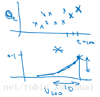
So it’s really taking the daily temperature multiply with this exponentially decay function, and then summing it up, and this become $v_{100}$

How many daily temperature is the averaging over?

$$(1 - \epsilon)^{\frac1{\epsilon}} = \frac1e \approx 0.35\tag1$$
$$\beta^{\frac1{1-\beta}} = \frac1e \approx 0.35$$

And so in other words, when $\beta = 0.9$, after $10(\frac1{1-0.9})$ days, the weight decays to less than $\frac13$ of the weight of the current day. And if $\beta = 0.98$, turn to that $0.98^{50} \approx \frac1e$. So we get the formule that we are averaging over $\frac1{1-\beta}$ day.

implemention exponontially weighted averages:

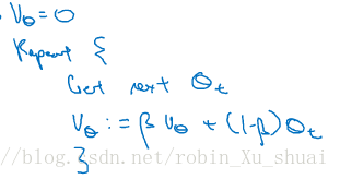
One of the advantage of this exponontially weighted averages is that it take very little memory, we just need to keep just one row number $V_{\theta}$ in computer memory and keep on overwriting it. And it’s really this reason, it just takes up one line of code basically and storage and memory for a single row number to compute this exponontially weighted averages.

It’s really not the best way, not the most accurate way to compute an average, if you were to compute a moving window, you can explicity sum over the last 10 days temperature just divide by 10 and that usually gives you a better estimate, but this disadvantage of that is need explicity keep all the temperatures and sum the last 10 days, it’s require more memory, and more complicated to implement.

So when we need to compute the average of a lot of variables, this is a very efficient way to do so both from the computation and the memory point of view.

5 - bias correction in exponentially weighted averages

We have learned how to implement exponentially weighted averages, There’s one technique detail called bias correction that can make your computation of these averages more accurately.

$$V_t = \beta V_{t-1} + (1-\beta)\theta_t$$

$$\begin{aligned} & V_0 = 0 \\ & V_1 = 0.02\theta_1 \\ & V_2 = 0.98V_1 + 0.02\theta_2=0.0196\theta_1+0.02\theta_2 \end{aligned}$$

so $V_1$ and $V_2$ are not very good estimate of the daily temperature for first and second day. These is a way to modify this estimate to make it much better, more accurate especially during the initial phase of your estimate.

$$V_t = \frac{\beta V_{t-1} + (1 - \beta)\theta_t}{1-\beta^{t}}$$

We notice that as t becomes large, $\beta^t$ will approach 0, which is why t is large enough, the bias correction make almost no different. And during the initial phase of learning, when we are still warming up estimates, bias correction can help get a better estimate.

In machine learning, most implementations of the exponentially weighted average we don’t bother to implement bias corrections.

6 - gradient descent with momentum

Momentum almost always works faster than the standard gradient descent. The basic idea is to compute an exponentially weighted averages of gradients, and then use that gradients to update the weights instead.

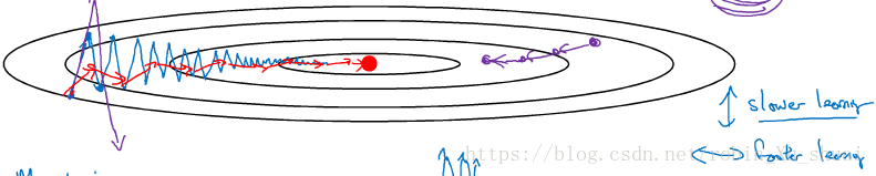
This up and down oscillations slows down gradient descent and prevent you from using a much larger learning rate. On the vertical axis we want step to be a bit slower, because we do not want those oscillations, but on the horizontal axis, we want faster learning. Here is we can do if we implement gradient descent with momentum.

Momentum:

on iteration t
1. compute dW, db on mini-batch
2. $V_{dW} = \beta V_{dW} + (1 - \beta)dW$
3. $V_{db} = \beta V_{db} + (1 - \beta)db$
4. $W = W - \alpha V_{dW}, b = b - \alpha V_{db}$

What this does is smooth the step of gradient descent, because we average over the oscillater gradient in the vertical direction so it’s become close to 0 by average positive and negative numbers. Whereas in the horizontal direction, the average in the horizontal will be pretty big. So our algorithm will take a more straightforward path.

---

Let’s look at detail how to implement:

thers are two hyperparameters, $\alpha, \beta$, the most common value for $\beta$ is 0.9, rougly average over the last 10 gradients.

$V_{dw} = 0, V_{db} = 0$

on iteration t
1. compute $dW$, $db$ on mini-batch
2. $V_{dW} = \beta V_{dW} + (1 - \beta)dW$
3. $V_{db} = \beta V_{db} + (1 - \beta)db$
4. $W = W - \alpha V_{dW}, b = b - \alpha V_{db}$

7 - RMSprop

We have seen how using momentum can speed up gradient descent. There is another algorithm called RMSprop, which stand for root mean square prop.

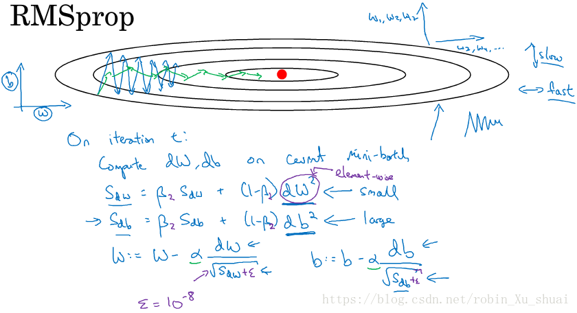
In order provides intuition of this algorithms, let’s say the vertical axis is the parameters b, and the horizontal axis is the parameter W, for the sake for intuition.So we want to slow down the learning in b direction, and speed up, or at least not slow down the learning in W direction.

Following is what RMSprop algorithm does to accomplish this:

on iteration t

1. compute $dW, db$ on current mini-batch
2. $S_{dw} = \beta S_{dw} + (1 - \beta)dW^2, S_{db} = \beta S_{db} + (1 - \beta)db^2$
3. $W = W - \alpha \frac{dW}{\sqrt{S_{dw}}+\epsilon}, b = b - \alpha \frac{db}{\sqrt{S_{db}}+\epsilon}$

Let’s gain some ituition about how this works. In the W direction, we want learning to go pretty fast, whereas in the b direction we want to slow down the oscillations, so what we hoping is that $S_{dw}$ will be small, whereas $S_{db}$ will be relatively large. And indeed, the derivatives are much larger in the b direction than in the W direction. **So $db^2$ will be relatively large, so $S_{db}$ will be relatively large, whereas compared to $dW$ will be smaller, $S_{dw}$ will be relatively smaller. So the effect of this is the update in b direction becomes small so that will help damp out the oscillations. **So you can therefore use a larger learning rate to get faster learning, speed up your learning algorithm.

8 - Adam optimization algorithm

The Adam optimization algorithm is basically taking momentum and RMSporp and putting them together.

Adam optimization algorithm

$V_{dw} = 0, V_{db} = 0, S_{dw} = 0, S_{db} = 0$

on iterations t:
1. compute $dw, db$ using mini-batch
2. $V_{dw} = \beta_1 V_{dw} + (1 - \beta_1)dw, \ V_{db} = \beta_1V_{db} + (1 - \beta_1)db$
3. $S_{dw} = \beta_2 S_{dw} + (1 - \beta_2)dw^2, \ S_{db} = \beta_2S_{db} + (1 - \beta_2)db^2$
4. $V_{dw}^{corrected} = \frac{V_{dw}}{1-\beta_1^t}, \ V_{db}^{corrected} = \frac{V_{db}}{1-\beta_1^t}$
5. $S_{dw}^{corrected} = \frac{S_{dw}}{1-\beta_2^t}, \ S_{db}^{corrected} = \frac{S_{db}}{1-\beta_2^t}$
6. $W = W - \alpha \frac{V_{dw}^{corrected}}{\sqrt{S_{dw}^{corrected}}+\epsilon}, b = b - \alpha \frac{V_{db}^{corrected}}{\sqrt{S_{db}^{corrected}}+\epsilon}$

This is a commonly used learning algorithm is proven to be very effective for many different neural networks of a very variety of architecture.

hyperparameters choice:

• $\alpha$: need to be tune
• $\beta_1 = 0.9$: $dw$
• $\beta_2 = 0.999$: $dw^2$
• $\epsilon = 10e-8$

Why does the term “Adam” comes from? “Adam” stands for Adaptive Momentum Estimation.

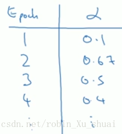
9 - learning rate decay

One of the things may speed up learning algorithm is to slowly reduce learning rate over time.

Suppose we are implementing mini-batch gradient descent, with a reasonably small mini-batch, maybe just 64 example, and as iterate, step will be a little bit noisy. The algorithm might just end up wandering around and never really converge, because we are using some fix value of $\alpha$ and there is some noise in different mini-batch.

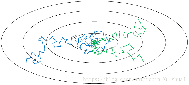
but if we were to slowly reduce learning rate, during the initial phases can have relatively faster learning, but then as $\alpha$ get smaller, the steps will be take smaller. So we can end up oscillating in a tightly region around the minimum rather than wandering far away. So the intuition behind slowly reduce $\alpha$ is that maybe during the initial steps of learning, we could afford to take much bigger steps, but as learning approach converges, need a slower learning rate to take smaller steps.

$$\alpha = \frac{1}{1+\text{decay-rate} * \text{epoch}}\alpha_0$$

when $\alpha_0 = 0.2, \text{decay-rate} = 1$

There are a few way other people use:

$$\alpha = 0.95^{\text{epoch}}\alpha_0$$
$$\alpha = \frac{k}{\sqrt{\text{epoch}}}\alpha_0\ \text{or}\ \frac{k}{\sqrt{t}}\alpha_0$$

or discrete learning rate.

Learning rate decay is a little bit lower down list in terms of the things we would to tuning.

10 - the problem of local optima

In the first picture, it looks like there are a lot of local optima, and it be easy for gradient descent or one of the other algorithm to get stuck in a local optimum rather than find its way to global optimum. It turn out that if you are plotting a figure like this in two dimensions, it’s easy to create plot like this with a lot of different local optima. And there low dimensional plots used to guide our intuition, but this intuition is not actually correct. It turn out if we create a neural network, most point of zero gradients are not local optima, instead the most point of zero gradient are saddle point. **So one of the lessons we learned from this is that a lot of intuition about low-dimensional spaces don’t transfer to very high-dimensional spaces. **Becasue we have 20000 parameters, and we much more likely to see saddle point than local optima.

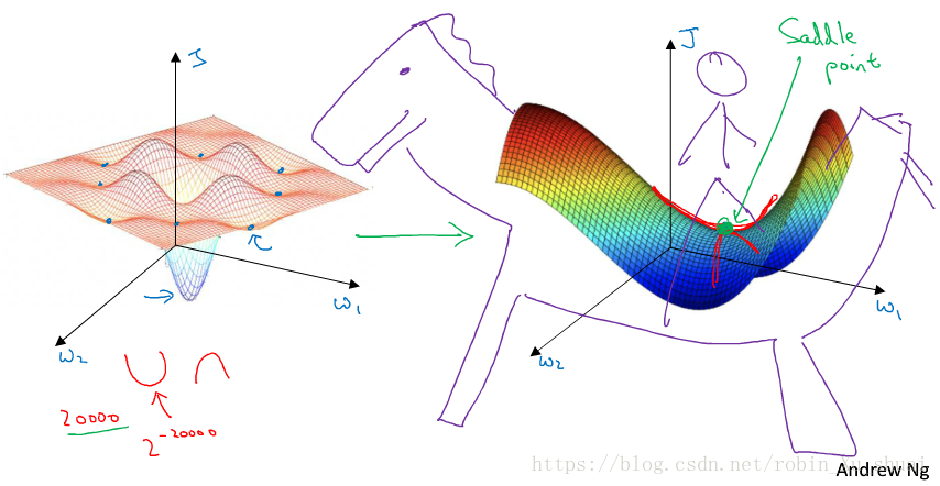
It turns out the plateaus can really slow down learning.

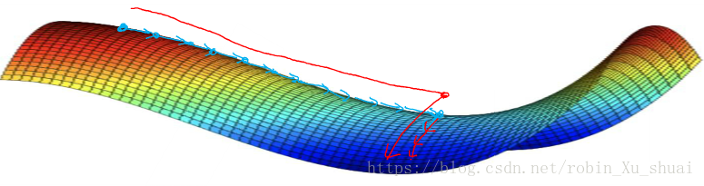
Plateaus is a region where the derivative is close to zero for a long time. So we need take away:

1. Unlikely to get stuck in a bad local optima, so long as we training a reasonably large neural network. so the cost function J is defined over a high dimensional space.
2. the plateaus can make learning slow, and this is where algorithms like momentum or RMSprop or Adam can really help learning algorithm and actually speed up the rate at which we could move down the plateaus and get off the plateaus.