DL notes07：GAN/DCGAN

GAN

Throughout most of this book, we have talked about how to make predictions. In some form or another, we used deep neural networks learned mappings from data points to labels. This kind of learning is called discriminative learning, as in, we’d like to be able to discriminate between photos cats and photos of dogs. Classifiers and regressors are both examples of discriminative learning. And neural networks trained by backpropagation have upended everything we thought we knew about discriminative learning on large complicated datasets. Classification accuracies on high-res images has gone from useless to human-level (with some caveats) in just 5-6 years. We will spare you another spiel about all the other discriminative tasks where deep neural networks do astoundingly well.

But there is more to machine learning than just solving discriminative tasks. For example, given a large dataset, without any labels, we might want to learn a model that concisely captures the characteristics of this data. Given such a model, we could sample synthetic data points that resemble the distribution of the training data. For example, given a large corpus of photographs of faces, we might want to be able to generate a new photorealistic image that looks like it might plausibly have come from the same dataset. This kind of learning is called generative modeling.

Until recently, we had no method that could synthesize novel photorealistic images. But the success of deep neural networks for discriminative learning opened up new possibilities. One big trend over the last three years has been the application of discriminative deep nets to overcome challenges in problems that we do not generally think of as supervised learning problems. The recurrent neural network language models are one example of using a discriminative network (trained to predict the next character) that once trained can act as a generative model.

In 2014, a breakthrough paper introduced Generative adversarial networks (GANs) Goodfellow.Pouget-Abadie.Mirza.ea.2014, a clever new way to leverage the power of discriminative models to get good generative models. At their heart, GANs rely on the idea that a data generator is good if we cannot tell fake data apart from real data. In statistics, this is called a two-sample test - a test to answer the question whether datasets X = { x 1 , … , x n } X=\{x_1,\ldots, x_n\} X={ x1​,…,xn​} and X ′ = { x 1 ′ , … , x n ′ } X'=\{x'_1,\ldots, x'_n\} X′={ x1′​,…,xn′​} were drawn from the same distribution. The main difference between most statistics papers and GANs is that the latter use this idea in a constructive way. In other words, rather than just training a model to say “hey, these two datasets do not look like they came from the same distribution”, they use the two-sample test to provide training signals to a generative model. This allows us to improve the data generator until it generates something that resembles the real data. At the very least, it needs to fool the classifier. Even if our classifier is a state of the art deep neural network.

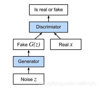
The GAN architecture is illustrated.As you can see, there are two pieces in GAN architecture - first off, we need a device (say, a deep network but it really could be anything, such as a game rendering engine) that might potentially be able to generate data that looks just like the real thing. If we are dealing with images, this needs to generate images. If we are dealing with speech, it needs to generate audio sequences, and so on. We call this the generator network. The second component is the discriminator network. It attempts to distinguish fake and real data from each other. Both networks are in competition with each other. The generator network attempts to fool the discriminator network. At that point, the discriminator network adapts to the new fake data. This information, in turn is used to improve the generator network, and so on.

The discriminator is a binary classifier to distinguish if the input $x$ is real (from real data) or fake (from the generator). Typically, the discriminator outputs a scalar prediction $o\in \mathbb{R}$ or input $\mathbf{x}$ such as using a dense layer with hidden size 1, and then applies sigmoid function to obtain the predicted probability $D(\mathbf{x})=1/(1+e^{-o})$ Assume the label $y$ for the true data is $1$ and $0$ for the fake data. We train the discriminator to minimize the cross-entropy loss, i.e.,
min ⁡ D { − y log ⁡ D ( x ) − ( 1 − y ) log ⁡ ( 1 − D ( x ) ) } \min_D \{ - y \log D(\mathbf x) - (1-y)\log(1-D(\mathbf x)) \} Dmin​{ −ylogD(x)−(1−y)log(1−D(x))}
For the generator, it first draws some parameter$\mathbf{z}\in {\mathbb{R}}^d$ from a source of randomness, e.g., a normal distribution $\mathbf{z}\sim \mathcal{N}(0,1)$ We often call $\mathbf{z}$ as the latent variable. It then applies a function to generate ${\mathbf{x}}^{\prime }=G(\mathbf{z})$ The goal of the generator is to fool the discriminator to classify ${\mathbf{x}}^{\prime }=G(\mathbf{z})$
as true data, i.e., we want $D(G(\mathbf{z}))\approx 1$ In other words, for a given discriminator $D$ , we update the parameters of the generator $G$ o maximize the cross-entropy loss when $y=0$ . i.e.,
$$\underset{G}{\max }$$