RNN学习笔记（五）-RNN 代码实现

RNN学习笔记（五）-RNN 代码实现

1.语言模型（LM）简述

做过NLP任务的童鞋应该都知道什么是语言模型，简单来说，如果我们把一句话s看做是由若干个(n个)词w组成的集合，那么这句话生成的概率就为：
$P(s)=p(w_1,w_2,...,w_n)=p(w_1)p(w_2|w_1)p(w_3|w_1,w_2)...p(w_n|w_1,...,w_{n-1})$
显然，右边的式子非常难以计算，它需要估算n个联合条件分布率。通常我们会做一些假设，比如，假设每个词的出现只依赖它的前一个词。那么上式就可以化简为：
$P(s)=p(w_1)p(w_2|w_1)p(w_3|w_2)...p(w_n|w_{n-1})$
如果依赖与前两个词：
$P(s)=p(w_1)p(w_2|w_1)p(w_3|w_1,w_2)...p(w_n|w_{n-2},w_{n-1})$
以上分别被称为2-Gram和3-Gram，对应的可以定义出4-Gram，5-Gram等等。前面关联的词越多，模型就越精确，相应的训练成本就越大。
在这里，为了简单起见，我们将通过RNN来训练一个2-Gram。即通过RNN来估计出每对单词的条件概率$p(w_i|w_j)$

2.RNN网络结构

训练样本（sentence）数为$N_s$，目标词典的word数量为$N_w$,每个单词使用one-hot表示（即该单词在词典中的Index），输入（出）层节点数$N_i=N_o=N_w$其中隐层节点数为$N_h$（通常为N_i的十分之一左右）。隐层节点激活函数为tanh，输出层节点激活函数为softmax。隐层存在一个递归边，每一时刻的输出乘以权值矩阵W后将作为下一时刻输入的一部分。
权值矩阵：
U：Input Layer->Hidden(t) Layer,大小为（$N_h×N_i$）
V：Hidden(t) Layer->Output Layer,大小为（$N_o×N_h$）
W：Hidden(t-1) Layer->Hidden(t) Layer,大小为（$N_h×N_h$）
$f_h$:隐层激活函数
$f_o$:输出层激活函数
$s_k(t)$:t时刻第k个隐层节点的输出值
$o_k(t)$:t时刻第k个输出层节点的输出值
$y_k$:第k个输出层节点的目标输出值（即学习signal）

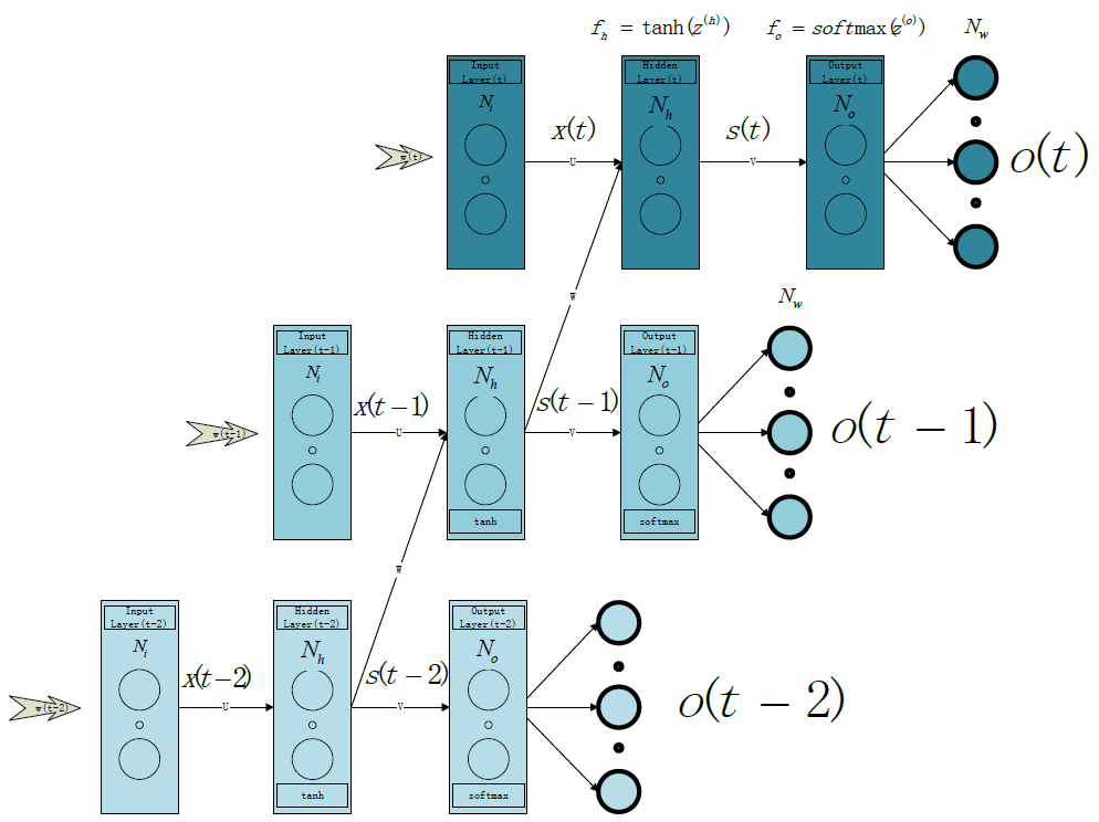
如上图所示，整个网络可以在时间上无限延展，每个时刻t网络都有一个对应的输入向量$x(t)$,一个隐层输出（状态）向量$s(t)$,一个输出向量$o(t)$。
输入向量$x(t)$和期望输出向量$y(t)$结构如下（假设输入的sentence由4个words组成）：

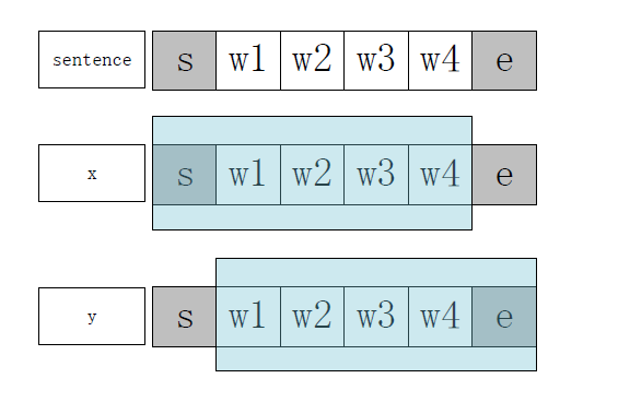
可以看到，y刚好相对于x有一个时刻的偏移，即：$y(t)=x(t+1)$
因此，t时刻的损失函数通过$y(t)$和$o(t)$即可求出。具体计算方法参见下边的小节。

3.python代码分析

这里我们使用python的Numpy包来实现，类名为RNNNumpy。另外代码中有中文注释，如果pydev中运行报错，在py文件最开始加上“#coding=utf-8”

3.0 主程序中的关键代码

3.0.1 文件读取

按行读取文件，每一行为一个句子(sentence)，并在每个句子的开头和结尾添加SENTENCE_START及SENTENCE_END word。

# with open('data/script.txt', 'rb') as f:
with open('data/script.txt', 'rb') as f:
    reader = csv.reader(f, skipinitialspace=True)
    reader.next()
    # Split full comments into sentences
    sentences = itertools.chain(*[nltk.sent_tokenize(x[0].decode('utf-8').lower()) for x in reader])
    # Append SENTENCE_START and SENTENCE_END
    sentences = ["%s %s %s" % (sentence_start_token, x, sentence_end_token) for x in sentences]
print "Parsed %d sentences." % (len(sentences))

3.0.2 分词及词频信息统计

vocabulary_size：词典的大小，即$N_w$。这里取训练语料经过分词后所有不重复词的数目；
tokenized_sentences：分词后的句子，每个句子由一个word的list组成，分词使用最简单的按空格
切分的方式，如果需要处理中文可以先使用中文专用的分词器切分语料；
word_freq：每个词在语料中出现的次数

# Tokenize the sentences into words
tokenized_sentences = [nltk.word_tokenize(sent) for sent in sentences]

# Count the word frequencies
word_freq = nltk.FreqDist(itertools.chain(*tokenized_sentences))
vocabulary_size = len(word_freq.items())

3.0.3 去除低频词、word转index

vocab：只存储词典中出现频率排名前$N_w-1$的词（相当于去掉了出现频率最低的词）
word_to_index：word到index的映射表

# Get the most common words and build index_to_word and word_to_index vectors
vocab = word_freq.most_common(vocabulary_size-1)
#将词典中所有的词（非重复）存储在index_to_word中
index_to_word = [x[0] for x in vocab]
#添加为登录词标记
index_to_word.append(unknown_token)
word_to_index = dict([(w,i) for i,w in enumerate(index_to_word)])

3.0.4 去除停用词

# Replace all words not in our vocabulary with the unknown token
for i, sent in enumerate(tokenized_sentences):
    tokenized_sentences[i] = [w if w in word_to_index else unknown_token for w in sent]

3.0.5 生成训练数据

X_train:即公式中的输入x，取每个sentence word index list的前T-1个元素，X_train中每一行存储的是每个句子从t=0时刻到t=T-2时刻的word index，T为该句子的长度；
y_train:即公式中的训练数据$y$，取每个sentence word index list的后T-1个元素(除去第一个元素)，y_train中每一行存储的是每个句子从t=1时刻到t=T-1时刻的word index；

# Create the training data
X_train = np.asarray([[word_to_index[w] for w in sent[:-1]] for sent in tokenized_sentences])
y_train = np.asarray([[word_to_index[w] for w in sent[1:]] for sent in tokenized_sentences])

3.0.6 构建模型类

model = RNNNumpy(vocabulary_size, hidden_dim=_HIDDEN_DIM)

3.0.7 模型训练

def train_with_sgd(model, X_train, y_train, learning_rate=0.005, nepoch=1, evaluate_loss_after=5):
    """
    Train RNN Model with SGD algorithm.

    Parameters
    ----------
    model : The model that will be trained
    X_train : input x
    y_train：期望输出值
    learning_rate：学习率
    nepoch：迭代次数
    evaluate_loss_after：loss值估计间隔，训练程序将每迭代evaluate_loss_after次进行一次loss值估计
    """
    # We keep track of the losses so we can plot them later
    losses = []
    num_examples_seen = 0
    #循环迭代训练，这个for循环每运行一次，就完成一次对所有数据的迭代
    for epoch in range(nepoch):
        # Optionally evaluate the loss
        if (epoch % evaluate_loss_after == 0):
            loss = model.calculate_loss(X_train, y_train)
            losses.append((num_examples_seen, loss))
            time = datetime.now().strftime('%Y-%m-%d-%H-%M-%S')
            print "%s: Loss after num_examples_seen=%d epoch=%d: %f" % (time, num_examples_seen, epoch, loss)
            # Adjust the learning rate if loss increases
            #如果当前一次loss值大于上一次，则调小学习率
            if (len(losses) > 1 and losses[-1][1] > losses[-2][1]):
                learning_rate = learning_rate * 0.5  
                print "Setting learning rate to %f" % learning_rate
            sys.stdout.flush()
            # ADDED! Saving model oarameters
            save_model_parameters_theano("./data/rnn-theano-%d-%d-%s.npz" % (model.hidden_dim, model.word_dim, time), model)
        # For each training example...
        #对所有训练数据执行一轮SGD算法迭代
        for i in range(len(y_train)):
            # One SGD step
            model.sgd_step(X_train[i], y_train[i], learning_rate)
            num_examples_seen += 1

3.0.8 辅助函数

辅助函数在utils.py中，这里不做过多解释，相信大家都能看懂：

def softmax(x):
    xt = np.exp(x - np.max(x))
    return xt / np.sum(xt)

def save_model_parameters_theano(outfile, model):
    U, V, W = model.U.get_value(), model.V.get_value(), model.W.get_value()
    np.savez(outfile, U=U, V=V, W=W)
    print "Saved model parameters to %s." % outfile

def load_model_parameters_theano(path, model):
    npzfile = np.load(path)
    U, V, W = npzfile["U"], npzfile["V"], npzfile["W"]
    model.hidden_dim = U.shape[0]
    model.word_dim = U.shape[1]
    model.U.set_value(U)
    model.V.set_value(V)
    model.W.set_value(W)
    print "Loaded model parameters from %s. hidden_dim=%d word_dim=%d" % (path, U.shape[0], U.shape[1])

3.1 RNN实现类RNNNumpy

3.1.1 初始化

    def __init__(self, word_dim, hidden_dim=100, bptt_truncate=4):
        """
        Instantiates the RNN class.

        Parameters
        ----------
        word_dim : 输入词向量的维度，如果是one hot，显然应该等于Input Layer 的结点数
        hidden_dim : 隐层的结点数
        bptt_truncate：BPTT反向传播的时间范围
        """

        # Assign instance variables
        self.word_dim = word_dim
        self.hidden_dim = hidden_dim
        self.bptt_truncate = bptt_truncate

        # Randomly initialize the network parameters
        self.U = np.random.uniform(-np.sqrt(1./word_dim), np.sqrt(1./word_dim), (hidden_dim, word_dim))
        self.V = np.random.uniform(-np.sqrt(1./hidden_dim), np.sqrt(1./hidden_dim), (word_dim, hidden_dim))
        self.W = np.random.uniform(-np.sqrt(1./hidden_dim), np.sqrt(1./hidden_dim), (hidden_dim, hidden_dim))

3.1.2 前向传播

前向传播对应的公式如下：
$f_h(x)=tanh(x)=\frac{e^x-e^{-x}} {e^x+e^{-x}}$
fo(x,z)=softmax(x)=